Maths refresher

The linear algebra, calculus, probability, statistics and logarithms that Chapters 1 and 2 lean on, stated properly and then run in NumPy.

This appendix is for readers who met vectors, derivatives and standard deviations once, in a first-year course, and have not touched them since: chemists, biologists and anyone whose maths is rusty. If you have a mathematics or physics degree, skip it; nothing here will be new. Nothing here is required reading before the episodes either. Each section opens with the episodes that use the idea, so you can come back when a formula or a line of NumPy stops you, read the one section you need, and return.

Every section is built the same way. First the theory: the definitions, stated precisely, and the results the episodes rely on, with a short proof where a proof is genuinely illuminating and a sketch or a reference where it is not. Then the same ideas in a few small NumPy cells that make them concrete. The cells run top to bottom, so copy any of them into a notebook and change the numbers. Each section ends with ★ self-checks and hidden solutions.

Definitions, theorems and propositions are numbered in order of appearance on this page. Proofs are collapsed; open them when you want to see why a statement holds, not just that it does.

import numpy as np
import pandas as pd

penguins = pd.read_csv("data/penguins.csv").dropna()
columns = ["bill_length_mm", "bill_depth_mm", "flipper_length_mm", "body_mass_g"]

Notation

Symbol	Meaning
\(\mathbb{R}\), \(\mathbb{R}^n\), \(\mathbb{R}^{m \times n}\)	the real numbers; vectors with \(n\) real entries; matrices with \(m\) rows and \(n\) columns
\(x_i\), \(A_{ij}\)	entry \(i\) of the vector \(x\); the entry of the matrix \(A\) in row \(i\), column \(j\)
\(x^\top\), \(A^\top\)	transpose: a column vector written as a row; rows and columns of \(A\) swapped
\(\operatorname{span}\), \(\dim\), \(\operatorname{rank}\)	the span of some vectors; the dimension of a space; the rank of a matrix
\(\operatorname{col}(A)\), \(\operatorname{null}(A)\)	column space and null space of a matrix
\(\lVert x \rVert\), \(\lVert x \rVert_1\)	Euclidean norm (length) of \(x\); the \(\ell_1\) norm \(\sum_i \lvert x_i \rvert\)
\(\sum_{i=1}^{n} x_i\)	the sum \(x_1 + x_2 + \cdots + x_n\); the limits are omitted when they are clear
\(f'(x)\), \(\partial L / \partial \theta_j\), \(\nabla L\)	derivative; partial derivative; gradient (the vector of all partial derivatives)
\(\Omega\), \(P(A)\), \(P(A \mid B)\)	sample space; probability of the event \(A\); probability of \(A\) given \(B\)
\(F_X\), \(p_X\), \(f_X\)	distribution function, probability mass function and density of a random variable \(X\)
\(\mathbb{E}[X]\), \(\operatorname{Var}(X)\), \(\operatorname{Cov}(X, Y)\)	expectation, variance and covariance
\(X \sim N(\mu, \sigma^2)\), \(\Phi\)	“\(X\) has the normal distribution with mean \(\mu\) and variance \(\sigma^2\)”; the standard normal distribution function
\(\bar{x}\), \(s^2\)	sample mean and sample variance of a list of numbers
\(\hat{y}\), \(\hat{\theta}\)	a prediction, an estimate; the hat marks a quantity computed from data
\(\arg\min_\theta L(\theta)\)	the value of \(\theta\) at which \(L\) is smallest

Lower-case letters (\(x\), \(w\), \(\theta\), \(\lambda\)) are vectors or scalars, and the text always says which; in this course a vector is a column by default, so \(x^\top w\) is a number and \(x w^\top\) is a matrix. Upper-case letters are matrices in the linear-algebra sections and random variables in the probability sections; the context always decides. Chapter 2 writes the intercept of a linear model as \(\theta_0\) and the feature weights as \(\theta_1, \ldots, \theta_p\); this appendix writes a general parameter vector as \(\theta = (\theta_1, \ldots, \theta_p)^\top\).

Vectors and vector spaces

Used in episode 1.2 (arrays), episode 2.2 (the linear model, and why duplicated features break it) and episode 2.4 (the norms behind ridge and lasso).

The vector you will meet most often in this course is the description of one sample: the four measurements of one penguin, or the handful of descriptors of one molecule. Each position in the list is one feature, and the order never changes, so position 3 always means “flipper length”. In NumPy a vector is a one-dimensional NumPy array.

penguin = penguins[columns].iloc[0].to_numpy()  # bill length, bill depth, flipper length (mm), body mass (g)
penguin, penguin.shape

(array([  39.1,   18.7,  181. , 3750. ]), (4,))

The shape (4,) says: one axis, four entries. What makes such lists useful is not the numbers themselves but two operations, adding two of them and scaling one by a number, and the rules those operations obey. The same rules hold for many other objects (spectra, functions, matrices), so mathematics states them once.

Definition 1

Vector space

A (real) vector space is a set \(V\) together with an addition, which gives \(u + v \in V\) for \(u, v \in V\), and a scalar multiplication, which gives \(\lambda v \in V\) for \(\lambda \in \mathbb{R}\) and \(v \in V\), such that for all \(u, v, w \in V\) and all \(\lambda, \mu \in \mathbb{R}\):

\(u + v = v + u\) and \((u + v) + w = u + (v + w)\);
there is a zero vector \(0 \in V\) with \(v + 0 = v\), and every \(v\) has a negative \(-v \in V\) with \(v + (-v) = 0\);
\(\lambda (u + v) = \lambda u + \lambda v\), \((\lambda + \mu) v = \lambda v + \mu v\) and \(\lambda (\mu v) = (\lambda \mu) v\);
\(1\, v = v\).

The elements of \(V\) are called vectors and the real numbers \(\lambda\) scalars.

The basic example is \(\mathbb{R}^n\), the lists of \(n\) real numbers, with addition and scaling done entry by entry; the space of penguin feature vectors is \(\mathbb{R}^4\). Matrices of a fixed shape form a vector space in the same way, and so do real-valued functions, with \((f + g)(x) = f(x) + g(x)\): every prediction function of a model is a vector in that sense. A non-example is instructive: the set of concentration vectors, whose entries are non-negative, is not a vector space, because \((1, 2)\) belongs to it and \(-1 \cdot (1, 2)\) does not.

p1, p2 = penguins[columns].iloc[:2].to_numpy()
p1 + p2, 0.5 * (p1 + p2)  # the average of two penguins is again a vector in R^4

(array([  78.6,   36.1,  367. , 7550. ]),
 array([  39.3 ,   18.05,  183.5 , 3775.  ]))

Definition 2

Subspace

A subspace of a vector space \(V\) is a subset \(U \subseteq V\) that is itself a vector space with the same addition and scalar multiplication.

Proposition 1

Subspace test

A subset \(U \subseteq V\) is a subspace if and only if \(0 \in U\) and \(U\) is closed under both operations: \(u + v \in U\) and \(\lambda u \in U\) for all \(u, v \in U\) and \(\lambda \in \mathbb{R}\).

ProofShow proof

First two consequences of the axioms. \(0\,v = (0 + 0)\,v = 0\,v + 0\,v\), and adding \(-(0\,v)\) to both sides gives \(0\,v = 0\). Then \(v + (-1)v = (1 - 1)v = 0\,v = 0\), so \((-1)v = -v\).

If \(U\) is a subspace, it is closed under the operations by definition, and its zero vector \(0_U\) satisfies \(0_U + 0_U = 0_U\); adding \(-0_U\) (in \(V\)) to both sides gives \(0_U = 0\), so \(0 \in U\). Conversely, if \(U\) contains \(0\) and is closed, the operations of \(V\) are operations on \(U\); every axiom holds in \(U\) because it holds in \(V\), the zero vector is in \(U\) by assumption, and the negative of \(u \in U\) is \((-1)u \in U\).

Linear combinations, independence and bases

Definition 3

Linear combination and span

A linear combination of vectors \(v_1, \ldots, v_k \in V\) is a vector \(\lambda_1 v_1 + \cdots + \lambda_k v_k\) with scalars \(\lambda_1, \ldots, \lambda_k\). The span of \(v_1, \ldots, v_k\) is the set of all their linear combinations; by the subspace test it is a subspace, and it is the smallest subspace containing all the \(v_i\).

Definition 4

Linear independence

Vectors \(v_1, \ldots, v_k\) are linearly independent if the only scalars with \(\lambda_1 v_1 + \cdots + \lambda_k v_k = 0\) are \(\lambda_1 = \cdots = \lambda_k = 0\). Otherwise they are linearly dependent; then at least one of them is a linear combination of the others (solve the equation for any \(v_j\) whose coefficient is non-zero).

Definition 5

Basis and dimension

A basis of \(V\) is a list \(b_1, \ldots, b_n\) of linearly independent vectors that spans \(V\). If \(V\) has a basis with \(n\) elements, \(V\) has dimension \(n\), written \(\dim V = n\).

Theorem 1

Bases and coordinates

Let \(V\) be a vector space with a basis \(b_1, \ldots, b_n\).

Every \(v \in V\) can be written as \(v = c_1 b_1 + \cdots + c_n b_n\) in exactly one way; the numbers \(c_1, \ldots, c_n\) are the coordinates of \(v\) in that basis.
Every basis of \(V\) has exactly \(n\) elements, so the dimension is well defined, and any \(n\) linearly independent vectors in \(V\) form a basis.
In \(\mathbb{R}^n\) the standard basis \(e_1, \ldots, e_n\), where \(e_j\) has a 1 in position \(j\) and zeros elsewhere, is a basis; so \(\dim \mathbb{R}^n = n\), and the coordinates of \(x\) in the standard basis are its entries.

ProofShow proof

Item 1: a representation exists because the basis spans \(V\). If \(v = \sum_i c_i b_i = \sum_i d_i b_i\), then \(\sum_i (c_i - d_i) b_i = 0\), and linear independence forces \(c_i = d_i\) for every \(i\). Item 3: \(x = \sum_j x_j e_j\) shows that the \(e_j\) span \(\mathbb{R}^n\), and \(\sum_j \lambda_j e_j = (\lambda_1, \ldots, \lambda_n)\) is zero only if every \(\lambda_j\) is. Item 2 rests on the exchange lemma: in a space spanned by \(n\) vectors, any linearly independent list has at most \(n\) elements. Applied in both directions to two bases it shows they have the same length; its proof is in any linear-algebra text and is not needed here.

In data terms, the columns of a feature matrix are vectors too: one entry per sample. If one feature is a linear combination of others, for instance the same mass recorded in grams and in kilograms, or a total that is the sum of its parts, the columns are linearly dependent and carry less information than their number suggests. NumPy’s matrix_rank (defined properly in the next section) counts how many columns are independent.

X4 = penguins[columns].to_numpy()
X5 = np.column_stack([X4, penguins["body_mass_g"].to_numpy() / 1000])  # the same mass again, in kg
X4.shape, np.linalg.matrix_rank(X4), X5.shape, np.linalg.matrix_rank(X5)

((333, 4), np.int64(4), (333, 5), np.int64(4))

Five columns, but only four independent ones: the kilogram column is \(1/1000\) times the gram column. The coefficients that show the dependence form a non-zero vector \(v\) with \(X_5 v = 0\):

v_dep = np.array([0, 0, 0, 1, -1000])  # 1 x (mass in g) - 1000 x (mass in kg)
np.abs(X5 @ v_dep).max()  # zero, up to floating-point rounding

np.float64(8.881784197001252e-14)

Exercise★☆☆

Which are subspaces?

Which of these subsets of \(\mathbb{R}^3\) are subspaces? (a) \(\{x : x_1 + x_2 + x_3 = 0\}\); (b) \(\{x : x_1 = 1\}\); (c) \(\{x : x_1 \ge 0\}\); (d) the span of \((1, 0, 0)\) and \((0, 1, 0)\).

SolutionShow solution

Use the subspace test. (a) Yes: it contains \(0\), and if two vectors have entries summing to zero, so do their sum and every multiple. (b) No: it does not contain \(0\). (c) No: \((1, 0, 0)\) is in it but \(-1 \cdot (1, 0, 0)\) is not, so it is not closed under scalar multiplication. (d) Yes: a span is always a subspace; this one is the plane \(x_3 = 0\), of dimension 2.

Exercise★★☆

A hidden dependence

A descriptor table for five hypothetical molecules has three columns: the number of carbon atoms, the number of other heavy atoms, and the total number of heavy atoms. Are the columns linearly independent? Find a non-zero vector \(v\) with \(Xv = 0\), and say what that means for a linear model fitted on all three columns.

SolutionShow solution

The total is the sum of the other two, so the columns are dependent and \(v = (1, 1, -1)\) gives \(Xv = 0\) for every row, whatever the molecules are.

counts = np.array([[6, 1], [2, 1], [7, 2], [10, 4], [3, 0]])  # carbon, other heavy atoms (made-up rows)
Xh = np.column_stack([counts, counts.sum(axis=1)])
np.linalg.matrix_rank(Xh), Xh @ np.array([1, 1, -1])

(np.int64(2), array([0, 0, 0, 0, 0]))

For a linear model this means the weights are not determined: adding any multiple of \(v\) to a weight vector changes no prediction, because \(X(\theta + t v) = X\theta\). The least-squares theorem in the derivatives section shows that the fit then has infinitely many solutions, which is one of the reasons regularisation exists (episode 2.4). Note that the dependence must be linear: a column holding the ratio of the first two would not lower the rank.

Matrices and linear maps

Used in episode 1.2 and episode 2.2 (the linear model and the normal equation).

Definition 6

Matrix and transpose

A matrix \(A \in \mathbb{R}^{m \times n}\) is a rectangular array of real numbers with \(m\) rows and \(n\) columns; its entry in row \(i\) and column \(j\) is \(A_{ij}\). The pair \((m, n)\) is its shape. The transpose \(A^\top \in \mathbb{R}^{n \times m}\) is the matrix with \((A^\top)_{ij} = A_{ji}\): rows become columns.

Stack the feature vectors of several samples as rows and you get the matrix that every scikit-learn model expects: one row per sample, one column per feature. This is the X / y convention, and it is worth fixing in your head now because every .fit(X, y) in the course relies on it.

X = penguins[columns].head(3).to_numpy()
X

array([[  39.1,   18.7,  181. , 3750. ],
       [  39.5,   17.4,  186. , 3800. ],
       [  40.3,   18. ,  195. , 3250. ]])

X.shape, X.T.shape

((3, 4), (4, 3))

Shape is always (rows, columns), that is (n_samples, n_features). X[0] is the first penguin’s feature vector; X[:, 3] is the body mass of every penguin; the transpose X.T has one row per feature and one column per penguin.

Products

Definition 7

Matrix–vector and matrix–matrix products

For \(A \in \mathbb{R}^{m \times n}\) and \(w \in \mathbb{R}^n\), the product \(Aw \in \mathbb{R}^m\) has entries \[ (Aw)_i = \sum_{j=1}^{n} A_{ij}\, w_j . \] For \(A \in \mathbb{R}^{m \times k}\) and \(B \in \mathbb{R}^{k \times n}\), the product \(AB \in \mathbb{R}^{m \times n}\) has entries \[ (AB)_{ij} = \sum_{l=1}^{k} A_{il}\, B_{lj} . \] The products are defined only when the inner dimensions agree: \(n\) in the first case, \(k\) in the second.

Proposition 2

Rules for products

Let \(A\), \(B\), \(C\) be matrices whose shapes make the products below defined. Then

\((m \times k)\) times \((k \times n)\) has shape \((m \times n)\): inner dimensions must match, outer dimensions remain;
\((AB)C = A(BC)\) and \(A(B + C) = AB + AC\);
\((AB)^\top = B^\top A^\top\);
in general \(AB \neq BA\), and one side may not even be defined.

ProofShow proof

Items 1 and 4 are immediate from the definition. Item 2 is a reindexing of finite sums. For item 3, by the definitions of transpose and product, \[ \big((AB)^\top\big)_{ij} = (AB)_{ji} = \sum_l A_{jl} B_{li} = \sum_l (B^\top)_{il} (A^\top)_{lj} = (B^\top A^\top)_{ij} . \]

Another way to read \(Aw\): it is the linear combination of the columns of \(A\) with coefficients \(w_1, \ldots, w_n\). Row by row it is one dot product per row (dot products are the subject of the next section): the sum of each feature times its weight for sample \(i\). A linear model predicts exactly this way, \(\hat{y} = X w\), so X @ w is LinearRegression.predict in one line, up to the intercept that predict adds.

w = np.array([0.1, -0.2, 0.05, 0.001])
X @ w

array([12.97, 13.57, 13.43])

np.sum(X[0] * w)  # the first entry, done by hand

np.float64(12.97)

The shapes must agree: (3, 4) @ (4,) gives (3,). If the number of weights does not match the number of columns, NumPy refuses, which is a useful error to see early. The matrix product you will see in episode 2.2 is \(X^\top X\), which by item 1 is square with one row and column per feature, and by item 3 is its own transpose.

(X.T @ X).shape

(4, 4)

Common mistake

* is not matrix multiplication

In NumPy X * w multiplies element by element (and broadcasts w across the rows); X @ w is the matrix product. Both run without error on the arrays above, and only one of them is what the linear model does. If a hand calculation disagrees with your code, check which operator you used.

Linear maps

Definition 8

Linear map

A function \(T : V \to W\) between vector spaces is linear if \(T(u + v) = T(u) + T(v)\) and \(T(\lambda v) = \lambda\, T(v)\) for all vectors \(u, v\) and scalars \(\lambda\).

Proposition 3

Matrices are linear maps

For every \(A \in \mathbb{R}^{m \times n}\) the map \(x \mapsto Ax\) from \(\mathbb{R}^n\) to \(\mathbb{R}^m\) is linear. Conversely, every linear map \(T : \mathbb{R}^n \to \mathbb{R}^m\) is of this form, with the matrix whose \(j\)-th column is \(T(e_j)\). Composing linear maps corresponds to multiplying their matrices: \(x \mapsto A(Bx)\) is \(x \mapsto (AB)x\).

ProofShow proof

Linearity of \(x \mapsto Ax\) is item 2 of the rules for products. Conversely, write \(x = \sum_j x_j e_j\); linearity gives \(T(x) = \sum_j x_j\, T(e_j)\), which is the matrix with columns \(T(e_j)\) applied to \(x\). The last statement is associativity, \(A(Bx) = (AB)x\).

x_a, x_b = np.array([1.0, 0.0, 2.0, 0.5]), np.array([0.0, 3.0, -1.0, 1.0])
np.allclose(X @ (2 * x_a + x_b), 2 * (X @ x_a) + X @ x_b)  # linearity, checked numerically

True

Column space, null space and rank

Definition 9

Column space, null space, rank

For \(A \in \mathbb{R}^{m \times n}\), the column space \(\operatorname{col}(A) = \{Ax : x \in \mathbb{R}^n\} \subseteq \mathbb{R}^m\) is the span of the columns of \(A\), and the null space \(\operatorname{null}(A) = \{x \in \mathbb{R}^n : Ax = 0\}\) is the set of vectors \(A\) sends to zero. Both are subspaces. The rank of \(A\) is \(\operatorname{rank}(A) = \dim \operatorname{col}(A)\), the largest number of linearly independent columns.

Theorem 2

Rank–nullity

For every \(A \in \mathbb{R}^{m \times n}\), \[ \operatorname{rank}(A) + \dim \operatorname{null}(A) = n . \] Moreover \(\operatorname{rank}(A) = \operatorname{rank}(A^\top)\), so \(\operatorname{rank}(A) \le \min(m, n)\).

ProofShow proof

A sketch of the first statement. Choose a basis \(u_1, \ldots, u_k\) of \(\operatorname{null}(A)\) and extend it (by the exchange lemma) to a basis \(u_1, \ldots, u_k, w_1, \ldots, w_r\) of \(\mathbb{R}^n\), so \(k + r = n\). Every \(Ax\) is a combination of the \(Aw_i\), because the \(Au_i\) are zero; and the \(Aw_i\) are independent, because \(A(\sum_i c_i w_i) = 0\) puts \(\sum_i c_i w_i\) in the null space, which forces every \(c_i\) to be zero. So \(\operatorname{rank}(A) = r = n - k\). The equality of row rank and column rank is a standard theorem that we use without proof.

The theorem turns into a statement about data. A feature matrix with \(p\) columns and rank \(r\) has a null space of dimension \(p - r\): that many independent directions in which the weights of a linear model can move without changing a single prediction. With more features than samples (\(p > n\)), the rank is at most \(n < p\), so such directions always exist. The kilogram column above is a one-dimensional example.

Proposition 4

The matrix XᵀX

For every \(X \in \mathbb{R}^{n \times p}\), \(\operatorname{null}(X^\top X) = \operatorname{null}(X)\). Consequently \(X^\top X\) is invertible if and only if the columns of \(X\) are linearly independent.

ProofShow proof

If \(Xv = 0\) then \(X^\top X v = 0\). Conversely, if \(X^\top X v = 0\) then \(0 = v^\top X^\top X v = (Xv)^\top (Xv) = \lVert Xv \rVert^2\), so \(Xv = 0\). The second statement combines this with the theorem on linear systems below (an \(n \times n\) matrix is invertible exactly when its null space is \(\{0\}\)) and the fact that \(Xv = \sum_j v_j\, x_{\cdot j}\) is a combination of the columns \(x_{\cdot j}\), so \(\operatorname{null}(X) = \{0\}\) says precisely that the columns are independent.

Identity, inverse, and why we `solve`

Definition 10

Identity and inverse

The identity matrix \(I_n \in \mathbb{R}^{n \times n}\) has ones on the diagonal and zeros elsewhere, so that \(I_n v = v\) for every \(v \in \mathbb{R}^n\). A square matrix \(A \in \mathbb{R}^{n \times n}\) is invertible if there is a matrix \(A^{-1}\) with \(A^{-1} A = A A^{-1} = I_n\); \(A^{-1}\) is then unique and is called the inverse of \(A\).

Theorem 3

Solving a linear system

Let \(A \in \mathbb{R}^{n \times n}\). The following are equivalent:

\(A\) is invertible;
for every \(b \in \mathbb{R}^n\) the equation \(A\theta = b\) has exactly one solution, namely \(\theta = A^{-1} b\);
the only solution of \(A\theta = 0\) is \(\theta = 0\), that is \(\operatorname{null}(A) = \{0\}\), that is the columns of \(A\) are linearly independent.

ProofShow proof

(1 ⇒ 2) If \(A\theta = b\) then multiplying on the left by \(A^{-1}\) gives \(\theta = A^{-1} b\), so there is at most one solution; and \(A(A^{-1} b) = b\), so there is at least one. (2 ⇒ 3) Take \(b = 0\): the unique solution is \(0\). (3 ⇒ 1) The \(n\) columns of \(A\) are independent, so by the theorem on bases they form a basis of \(\mathbb{R}^n\) and span it. Hence each \(e_j = A b_j\) for some \(b_j\); the matrix \(B\) with columns \(b_j\) satisfies \(AB = I_n\). Moreover \(A(BA - I_n) = (AB)A - A = 0\), so every column of \(BA - I_n\) solves \(A\theta = 0\) and is zero by item 3; hence \(BA = I_n\) as well, and \(B = A^{-1}\).

The theorem is why the normal equation of linear regression is usually written as \(\theta = (X^\top X)^{-1} X^\top y\). It is not how it is computed. Forming an inverse explicitly is slower and loses precision, so numerical code asks NumPy to solve the equation directly: np.linalg.solve(A, b) returns the \(\theta\) that satisfies \(A\theta = b\) without ever building \(A^{-1}\).

A = np.array([[2.0, 1.0], [1.0, 3.0]])
b = np.array([3.0, 5.0])
theta = np.linalg.solve(A, b)
theta, A @ theta  # the second value should be b again

(array([0.8, 1.4]), array([3., 5.]))

The check A @ theta returning b is the whole story: solve found the \(\theta\) that makes the equation true. scikit-learn’s LinearRegression uses a least-squares solver that also copes with dependent columns, but the idea is the same.

Exercise★☆☆

Read the shapes

A feature matrix has 200 samples and 5 features. What are the shapes of X, X.T, X @ w (for a weight vector w with one weight per feature) and X.T @ X? What is the largest rank X can have?

SolutionShow solution

X is (200, 5); X.T is (5, 200); X @ w is (200,), one prediction per sample; X.T @ X is (5, 200) @ (200, 5), so (5, 5), one row and column per feature. The rule is item 1 of the rules for products: inner dimensions must match, outer dimensions remain. By rank–nullity the rank is at most \(\min(200, 5) = 5\), reached exactly when the five columns are linearly independent.

Exercise★☆☆

One dot product per row

Without running code, compute M @ v for M = [[1, 2], [3, 4], [5, 6]] and v = [10, 1]. Then check with NumPy.

SolutionShow solution

Row by row: \(1 \times 10 + 2 \times 1 = 12\), \(3 \times 10 + 4 \times 1 = 34\), \(5 \times 10 + 6 \times 1 = 56\). Equivalently, \(10\) times the first column plus \(1\) times the second.

M = np.array([[1, 2], [3, 4], [5, 6]])
v = np.array([10, 1])
M @ v

array([12, 34, 56])

Each output entry is the dot product of one row of M with v, which is why the result has one entry per row (shape (3,)).

Inner products, norms and distances

Used in episode 2.4 (the penalties of ridge and lasso), episode 2.5 (nearest neighbours) and episode 2.6 (feature scaling).

Definition 11

Dot product, Euclidean norm, distance

For \(a, b \in \mathbb{R}^n\) the dot product (or standard inner product) is \[ a \cdot b = \sum_{i=1}^{n} a_i b_i = a^\top b , \] the Euclidean norm (length) of \(a\) is \(\lVert a \rVert = \sqrt{a \cdot a} = \sqrt{\sum_i a_i^2}\), and the Euclidean distance between \(a\) and \(b\) is \(d(a, b) = \lVert a - b \rVert\).

Proposition 5

Elementary properties

For all \(a, b, c \in \mathbb{R}^n\) and scalars \(\lambda\): \(a \cdot b = b \cdot a\); \((\lambda a + c) \cdot b = \lambda (a \cdot b) + c \cdot b\); \(\lVert \lambda a \rVert = |\lambda| \, \lVert a \rVert\); and \(\lVert a \rVert \ge 0\) with equality only when \(a = 0\).

All four follow directly from the definition as a sum, and they are used silently in every argument below. The result that gives the dot product its geometric meaning is the following inequality.

Theorem 4

Cauchy–Schwarz inequality

For all \(a, b \in \mathbb{R}^n\), \[ |a \cdot b| \le \lVert a \rVert \, \lVert b \rVert , \] with equality if and only if one of the vectors is a scalar multiple of the other.

ProofShow proof

If \(b = 0\) both sides are zero. Otherwise, for every real \(t\) the squared length \(\lVert a - t b \rVert^2\) is non-negative, and expanding it with the elementary properties gives \[ 0 \le \lVert a - t b \rVert^2 = \lVert a \rVert^2 - 2t\,(a \cdot b) + t^2 \lVert b \rVert^2 . \] Choose \(t = (a \cdot b) / \lVert b \rVert^2\), the value that makes the right-hand side smallest. Then \(0 \le \lVert a \rVert^2 - (a \cdot b)^2 / \lVert b \rVert^2\), which rearranges to the inequality. Equality holds exactly when \(\lVert a - t b \rVert = 0\), that is when \(a = t b\).

Definition 12

Angle, cosine similarity, orthogonality

For non-zero \(a, b\), the cosine similarity is \(\cos\varphi = \dfrac{a \cdot b}{\lVert a \rVert \, \lVert b \rVert}\). By the Cauchy–Schwarz inequality it lies in \([-1, 1]\), so it is the cosine of a unique angle \(\varphi \in [0, \pi]\) between the two vectors. Vectors with \(a \cdot b = 0\) are orthogonal, written \(a \perp b\).

Proposition 6

Pythagoras and orthogonal projection

If \(a \perp b\) then \(\lVert a + b \rVert^2 = \lVert a \rVert^2 + \lVert b \rVert^2\).
Let \(b \neq 0\). The vector \(p = \dfrac{a \cdot b}{\lVert b \rVert^2}\, b\) is the only multiple of \(b\) with \((a - p) \perp b\), and it is the point of the line through \(b\) closest to \(a\): \(\lVert a - t b \rVert \ge \lVert a - p \rVert\) for every real \(t\), with equality only at \(p\). It is called the orthogonal projection of \(a\) onto the line through \(b\).

ProofShow proof

Item 1: expand \(\lVert a + b \rVert^2 = \lVert a \rVert^2 + 2\, a \cdot b + \lVert b \rVert^2\) and use \(a \cdot b = 0\). Item 2: \((a - s b) \cdot b = a \cdot b - s \lVert b \rVert^2\) is zero exactly for \(s = (a \cdot b) / \lVert b \rVert^2\), which gives \(p\). For any \(t\), \(a - t b = (a - p) + (p - t b)\), and \(p - tb\) is a multiple of \(b\), hence orthogonal to \(a - p\); by item 1, \(\lVert a - t b \rVert^2 = \lVert a - p \rVert^2 + \lVert p - t b \rVert^2 \ge \lVert a - p \rVert^2\), with equality only when \(tb = p\).

Written as a sum, the dot product looks like bookkeeping. The theorem and the definition make it geometry: \(a \cdot b = \lVert a \rVert \, \lVert b \rVert \cos\varphi\), so the dot product measures how much two vectors point the same way.

a = np.array([3.0, 4.0])
b = np.array([4.0, 3.0])
a @ b, np.sum(a * b)  # the same number two ways

(np.float64(24.0), np.float64(24.0))

The norm is Pythagoras in as many dimensions as you like, and NumPy computes it with np.linalg.norm.

np.linalg.norm(a), np.sqrt(a @ a)

(np.float64(5.0), np.float64(5.0))

Divide the dot product by both lengths and you are left with \(\cos\varphi\): \(1\) when the vectors point the same way, \(0\) when they are perpendicular, \(-1\) when they are opposite. For \(a = (3, 4)\) and \(b = (4, 3)\) the angle is small.

cos_phi = (a @ b) / (np.linalg.norm(a) * np.linalg.norm(b))
cos_phi, np.degrees(np.arccos(cos_phi))

(np.float64(0.96), np.float64(16.260204708311967))

The projection of \(a\) onto the line through \(b\), and a check that what is left over is orthogonal to \(b\):

p = (a @ b) / (b @ b) * b
p, (a - p) @ b  # the second number is zero up to rounding

(array([3.84, 2.88]), np.float64(8.881784197001252e-16))

The number \(a \cdot b / \lVert b \rVert\) is the signed length of that projection, the shadow \(a\) casts on the line through \(b\). So X @ w computes, for every row \(x_i\), the shadow length of \(x_i\) on the direction of \(w\), multiplied by \(\lVert w \rVert\): a linear model scores each sample by how far it extends along one direction in feature space. Cosine similarity comes back when you compare molecular fingerprints in Part II.

Norms in general

Definition 13

Norm

A norm on a vector space \(V\) is a function \(v \mapsto \lVert v \rVert\) with, for all \(u, v \in V\) and scalars \(\lambda\):

\(\lVert v \rVert \ge 0\), with equality only for \(v = 0\);
\(\lVert \lambda v \rVert = |\lambda| \, \lVert v \rVert\);
\(\lVert u + v \rVert \le \lVert u \rVert + \lVert v \rVert\) (the triangle inequality).

Proposition 7

Two norms on ℝⁿ

The Euclidean norm \(\lVert x \rVert = \sqrt{\sum_i x_i^2}\) and the \(\ell_1\) norm \(\lVert x \rVert_1 = \sum_i |x_i|\) are both norms on \(\mathbb{R}^n\). Consequently the Euclidean distance satisfies \(d(x, z) \le d(x, y) + d(y, z)\) for all \(x, y, z\).

ProofShow proof

Items 1 and 2 are immediate for both. For the triangle inequality of the Euclidean norm, \(\lVert a + b \rVert^2 = \lVert a \rVert^2 + 2\, a \cdot b + \lVert b \rVert^2 \le \lVert a \rVert^2 + 2 \lVert a \rVert \lVert b \rVert + \lVert b \rVert^2 = (\lVert a \rVert + \lVert b \rVert)^2\) by Cauchy–Schwarz. For \(\ell_1\) it follows from \(|a_i + b_i| \le |a_i| + |b_i|\) summed over \(i\). For the distance, apply the triangle inequality to \(a = x - y\) and \(b = y - z\).

The two norms measure size differently, and that is the whole difference between the two regularised regressions of episode 2.4: ridge penalises \(\alpha \lVert \theta \rVert^2\), the squared Euclidean norm of the weights, which shrinks all of them smoothly; lasso penalises \(\alpha \lVert \theta \rVert_1\), which can set some exactly to zero.

r = np.array([3.0, -4.0])
np.linalg.norm(r), np.linalg.norm(r, 1), np.abs(r).sum()

(np.float64(5.0), np.float64(7.0), np.float64(7.0))

Distance between two samples

np.linalg.norm(a - b)

np.float64(1.4142135623730951)

The Euclidean distance is what k-nearest neighbours (kNN) uses to decide which training samples are “nearest” to a new one, and it is where units come in. Take one penguin of each species and compute the three pairwise distances on the raw measurements.

three = penguins.groupby("species").head(1)
three[["species"] + columns]

index	species	bill_length_mm	bill_depth_mm	flipper_length_mm	body_mass_g
0	Adelie	39.1	18.7	181.0	3750.0
152	Gentoo	46.1	13.2	211.0	4500.0
276	Chinstrap	46.5	17.9	192.0	3500.0

P = three[columns].to_numpy()
raw = np.array([[np.linalg.norm(p - q) for q in P] for p in P])
pd.DataFrame(raw, index=three["species"], columns=three["species"]).round(0)

species	Adelie	Gentoo	Chinstrap
species	index	index	index
Adelie	0.0	751.0	250.0
Gentoo	751.0	0.0	1000.0
Chinstrap	250.0	1000.0	0.0

The distances are 250, 750 and 1000: almost exactly the differences in body mass in grams. The bills differ by a few millimetres and the flippers by a few tens, and those numbers are tiny next to hundreds of grams, so they contribute nothing. Distance on raw features is a body-mass ranking in disguise.

feature scaling fixes this by putting every feature on the same footing. Standardise each column (subtract its mean, divide by its standard deviation; see the statistics section) and compute the distances again.

Z = (penguins[columns] - penguins[columns].mean()) / penguins[columns].std()
Pz = Z.loc[three.index].to_numpy()
scaled = np.array([[np.linalg.norm(p - q) for q in Pz] for p in Pz])
pd.DataFrame(scaled, index=three["species"], columns=three["species"]).round(2)

species	Adelie	Gentoo	Chinstrap
species	index	index	index
Adelie	0.00	3.86	1.65
Gentoo	3.86	0.00	3.01
Chinstrap	1.65	3.01	0.00

Now all four measurements count, and the answer changes: on raw numbers the Gentoo’s nearest neighbour was the Adelie (750 g apart); after scaling it is the Chinstrap. The Chinstrap’s bill is almost exactly as long as the Gentoo’s (46.5 against 46.1 mm) and its flippers are closer (192 against 211 mm, where the Adelie has 181), and those millimetre differences finally count once the grams no longer swamp them. A kNN classifier would have flipped its vote. This is why scaling is part of the model, not a cosmetic step, and why episode 2.6 puts it inside a pipeline fitted on the training set only.

Exercise★☆☆

Dot product and distance by hand

For \(a = (1, 2, 2)\) and \(b = (2, 0, 0)\), compute \(a \cdot b\), \(\lVert a \rVert\), \(\lVert b \rVert\), \(\cos\varphi\), the projection of \(a\) onto the line through \(b\), and the Euclidean distance \(d(a, b)\). Then check with NumPy.

SolutionShow solution

\(a \cdot b = 2 + 0 + 0 = 2\); \(\lVert a \rVert = \sqrt{1 + 4 + 4} = 3\); \(\lVert b \rVert = 2\); \(\cos\varphi = 2 / (3 \times 2) = 1/3\); the projection is \((2/4)\, b = (1, 0, 0)\); \(d(a, b) = \sqrt{(1-2)^2 + 2^2 + 2^2} = \sqrt{9} = 3\).

a3 = np.array([1.0, 2.0, 2.0])
b3 = np.array([2.0, 0.0, 0.0])
a3 @ b3, np.linalg.norm(a3), np.linalg.norm(b3), (a3 @ b3) / (b3 @ b3) * b3, np.linalg.norm(a3 - b3)

(np.float64(2.0),
 np.float64(3.0),
 np.float64(2.0),
 array([1., 0., 0.]),
 np.float64(3.0))

A cosine of \(1/3\) means the vectors point in broadly different directions (about 71°). Scaling a vector by a positive factor changes distances but not angles: \((2, 4, 4)\) makes the same angle with \(b\) as \((1, 2, 2)\) does. A negative factor turns the angle \(\varphi\) into \(\pi - \varphi\).

Exercise★★☆

Where Cauchy–Schwarz bites

Suppose someone reports a cosine similarity of \(1.04\) between two molecular fingerprints. Without seeing the fingerprints, what can you say? And if two non-zero vectors have cosine similarity exactly \(-1\), what is the relationship between them?

SolutionShow solution

A cosine similarity above \(1\) is impossible: by the Cauchy–Schwarz inequality \(|a \cdot b| \le \lVert a \rVert \lVert b \rVert\), so the ratio lies in \([-1, 1]\). The number is a bug (most often a dot product divided by the wrong norms, or norms computed on different vectors). A cosine of exactly \(-1\) is the equality case with a negative constant: \(a = \lambda b\) with \(\lambda < 0\), so the vectors point in exactly opposite directions.

Derivatives and gradients

Used in episode 2.2 (fitting by gradient descent) and every neural network from Chapter 4 on.

Definition 14

Derivative

A function \(f : \mathbb{R} \to \mathbb{R}\) is differentiable at \(x\) if the limit \[ f'(x) = \lim_{h \to 0} \frac{f(x + h) - f(x)}{h} \] exists; \(f'(x)\) is the derivative of \(f\) at \(x\). Geometrically it is the slope of the tangent line to the graph of \(f\) at \(x\); physically it is the rate at which \(f\) changes per unit change in \(x\).

Proposition 8

Rules of differentiation

Where the functions involved are differentiable:

power rule: \(\dfrac{d}{dx} x^k = k x^{k-1}\) for every real \(k\) (and \(x > 0\) when \(k\) is not an integer);
linearity: \(\dfrac{d}{dx}\big(c\, g(x) + u(x)\big) = c\, g'(x) + u'(x)\) for every constant \(c\);
product rule: \(\dfrac{d}{dx}\big(g(x)\, u(x)\big) = g'(x)\, u(x) + g(x)\, u'(x)\).

Theorem 5

Chain rule

If \(g\) is differentiable at \(x\) and \(f\) is differentiable at \(g(x)\), then \(f \circ g\) is differentiable at \(x\) and \[ \frac{d}{dx} f\big(g(x)\big) = f'\big(g(x)\big)\, g'(x) : \] the outer derivative, evaluated at the inner value, times the inner derivative.

The chain rule is the one that matters for machine learning, because a loss is always “a function of the prediction, which is a function of the parameters”. Its proof is in any calculus text; the idea is that for small \(h\), \(g(x + h) \approx g(x) + g'(x) h\), and then \(f\) of that is approximately \(f(g(x)) + f'(g(x))\, g'(x)\, h\).

The definition is also a way to check a derivative numerically. Pick a small \(h\) and compute the ratio; the symmetric version \((f(x+h) - f(x-h)) / 2h\) is more accurate. Here the rules give \(f'(x) = 2x - 3\) for \(f(x) = x^2 - 3x\), and the finite difference agrees.

def f(x):
    return x**2 - 3 * x


x0, h = 2.5, 1e-6
(f(x0 + h) - f(x0 - h)) / (2 * h), 2 * x0 - 3  # numeric, exact

(2.000000000279556, 2.0)

A loss curve and its tangent

Suppose a one-parameter model \(\hat{y} = w x\) fitted to three points. The mean squared error (MSE) as a function of \(w\) is a curve, and the derivative at any \(w\) is the slope of the tangent there.

x = np.array([1.0, 2.0, 3.0])
y = np.array([2.0, 4.0, 5.0])


def loss(w):
    return np.mean((y - w * x) ** 2)


w0 = 0.8
slope = (loss(w0 + h) - loss(w0 - h)) / (2 * h)
loss(w0), slope

(np.float64(4.653333333333332), np.float64(-9.199999999598418))

import matplotlib.pyplot as plt

ws = np.linspace(0, 3.2, 200)
span = np.linspace(w0 - 0.6, w0 + 0.6, 2)
fig, ax = plt.subplots()
ax.plot(ws, [loss(w) for w in ws], label="loss L(w)")
ax.plot(span, loss(w0) + slope * (span - w0), linestyle="--", label=f"tangent at w = {w0}")
ax.scatter([w0], [loss(w0)], zorder=3)
ax.set(xlabel="weight w", ylabel="mean squared error", title="A 1-D loss curve and its tangent")
ax.legend()
plt.show()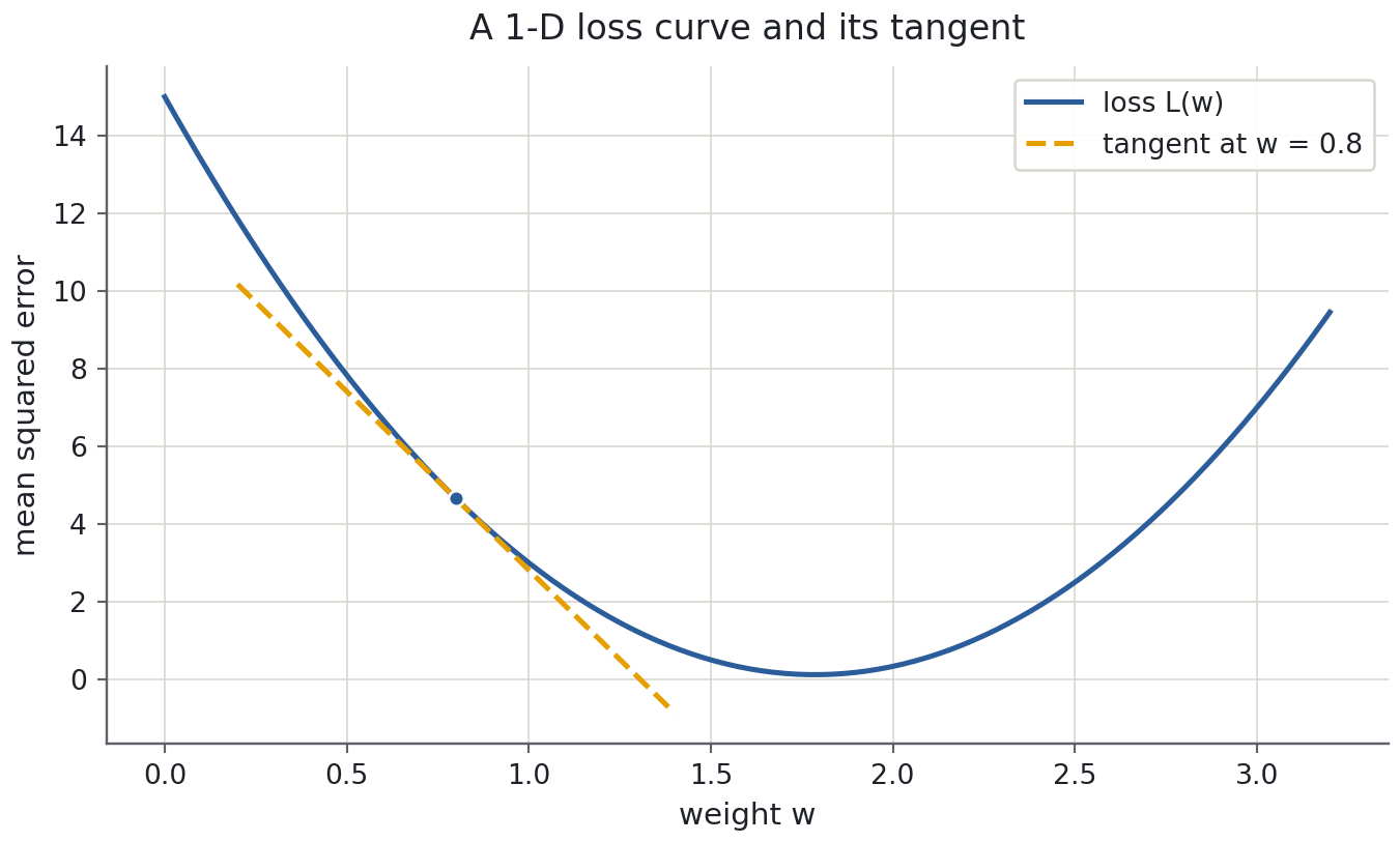

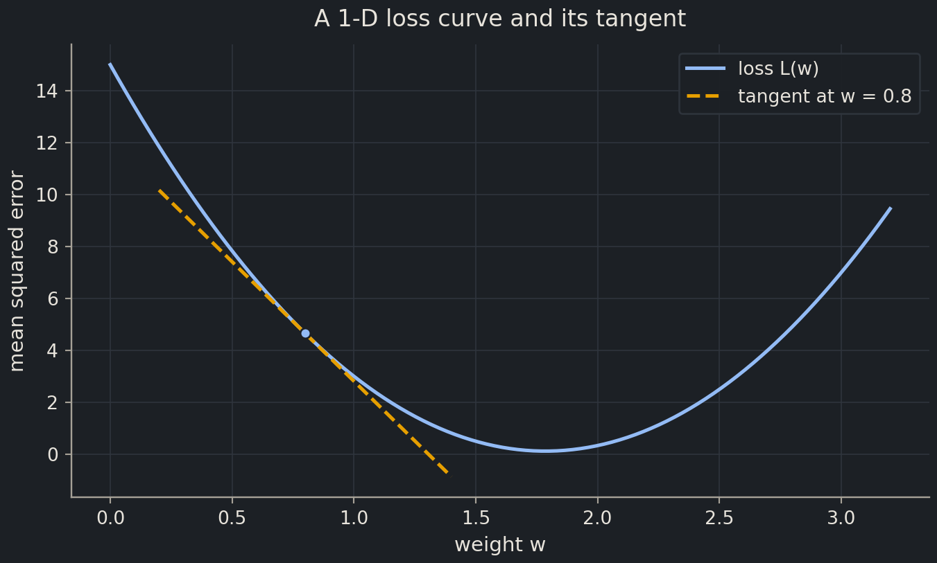
A U-shaped loss curve, mean squared error against the weight w, with a dot on the left arm at w = 0.8 and a dashed tangent line through it sloping steeply downwards to the right. The minimum of the curve is near w = 1.8.

At \(w = 0.8\) the slope is negative: the loss falls if \(w\) increases. At the bottom of the bowl the slope is zero, and to the right it is positive. So the sign of the derivative tells you which way to move to reduce the loss, and its size tells you how steep the curve is. That is all gradient descent needs, and the boxes below make it precise for many parameters.

Several parameters: partial derivatives and the gradient

Definition 15

Partial derivative and gradient

For \(L : \mathbb{R}^p \to \mathbb{R}\), the partial derivative \(\partial L / \partial \theta_j\) at \(\theta\) is the ordinary derivative of the one-variable function \(t \mapsto L(\theta_1, \ldots, \theta_j + t, \ldots, \theta_p)\) at \(t = 0\): all other coordinates are held fixed. The gradient is the column vector of all partial derivatives, \[ \nabla L(\theta) = \Big( \frac{\partial L}{\partial \theta_1}, \ldots, \frac{\partial L}{\partial \theta_p} \Big)^{\!\top} \in \mathbb{R}^p . \]

Theorem 6

The gradient is the direction of steepest ascent

Let \(L\) be differentiable at \(\theta\) (it suffices that all partial derivatives exist and are continuous near \(\theta\)), and let \(u \in \mathbb{R}^p\) be a unit vector. The rate of change of \(L\) at \(\theta\) in the direction \(u\) is \[ \frac{d}{dt} L(\theta + t u) \Big|_{t = 0} = \nabla L(\theta) \cdot u . \] If \(\nabla L(\theta) \ne 0\), this rate is largest when \(u = \nabla L(\theta) / \lVert \nabla L(\theta) \rVert\) and smallest (most negative) when \(u = -\nabla L(\theta) / \lVert \nabla L(\theta) \rVert\).

ProofShow proof

The first statement is the multivariable chain rule, which we use without proof: \(\frac{d}{dt} L(\theta + tu) = \sum_j \frac{\partial L}{\partial \theta_j} u_j\). For the second, Cauchy–Schwarz gives \(|\nabla L \cdot u| \le \lVert \nabla L \rVert \, \lVert u \rVert = \lVert \nabla L \rVert\), with equality exactly when \(u\) is a multiple of \(\nabla L\); the sign of the multiple decides between the maximum and the minimum.

Theorem 7

First-order condition for a minimum

If \(L\) is differentiable and \(\theta^\ast\) is a local minimum of \(L\), then \(\nabla L(\theta^\ast) = 0\).

ProofShow proof

Fix \(j\) and let \(g(t) = L(\theta^\ast + t e_j)\), where \(e_j\) is the \(j\)-th standard basis vector. Then \(g\) has a local minimum at \(t = 0\), so for small \(h > 0\) both \((g(h) - g(0))/h \ge 0\) and \((g(-h) - g(0))/(-h) \le 0\). Letting \(h \to 0\) gives \(g'(0) \ge 0\) and \(g'(0) \le 0\), so \(\partial L / \partial \theta_j = g'(0) = 0\). As \(j\) was arbitrary, the whole gradient vanishes.

The condition is necessary, not sufficient: a maximum or a saddle point also has zero gradient. For the losses of this course a separate argument (like the one for least squares below) shows that the stationary points found are minima.

Definition 16

Gradient descent

Given a differentiable loss \(L\), a starting point \(\theta_0\) and a learning rate \(\eta > 0\), gradient descent is the iteration \[ \theta_{k+1} = \theta_k - \eta\, \nabla L(\theta_k), \qquad k = 0, 1, 2, \ldots \]

By the steepest-ascent theorem each step moves in the direction in which the loss decreases fastest, and by the first-order condition the iteration stops changing exactly at points where the gradient vanishes, which includes every minimum. Here is the gradient of a two-parameter function at the origin, by finite differences and then by the rules.

def g(a, b):
    return (a - 1) ** 2 + 2 * (b + 2) ** 2


grad = np.array([
    (g(0 + h, 0) - g(0 - h, 0)) / (2 * h),  # dg/da at (0, 0)
    (g(0, 0 + h) - g(0, 0 - h)) / (2 * h),  # dg/db at (0, 0)
])
grad.round(4)

array([-2.,  8.])

By the rules, \(\partial g/\partial a = 2(a - 1)\) and \(\partial g/\partial b = 4(b + 2)\), which at \((0, 0)\) give \((-2, 8)\). Twenty steps of gradient descent walk from the origin to within about 0.01 of the minimum at \((1, -2)\), where both partials are zero.

theta, eta = np.array([0.0, 0.0]), 0.1
for step in range(20):
    grad = np.array([2 * (theta[0] - 1), 4 * (theta[1] + 2)])
    theta = theta - eta * grad
theta.round(3)

array([ 0.988, -2.   ])

Least squares

The loss of linear regression is simple enough that the minimisers can be described exactly. This is the result that episode 2.2 derives line by line in its deep dive.

Theorem 8

Least squares and the normal equations

Let \(X \in \mathbb{R}^{n \times p}\), \(y \in \mathbb{R}^n\), and \(L(\theta) = \frac{1}{n} \lVert y - X\theta \rVert^2\). Then

\(\nabla L(\theta) = -\dfrac{2}{n} X^\top (y - X\theta)\);
\(\theta\) minimises \(L\) if and only if it satisfies the normal equations \(X^\top X \theta = X^\top y\);
if the columns of \(X\) are linearly independent, the minimiser is unique and equals \(\hat{\theta} = (X^\top X)^{-1} X^\top y\). If they are dependent, the minimisers form a whole affine family \(\hat{\theta} + \operatorname{null}(X)\).

ProofShow proof

Item 1: expanding the squared norm with the rules for products, \(n L(\theta) = y^\top y - 2\theta^\top X^\top y + \theta^\top X^\top X \theta\). The gradient of \(\theta^\top c\) is \(c\), and the gradient of \(\theta^\top M \theta\) for a symmetric matrix \(M\) is \(2 M \theta\) (differentiate the double sum \(\sum_{i,j} \theta_i M_{ij} \theta_j\) coordinate by coordinate). With \(c = X^\top y\) and \(M = X^\top X\) this gives \(n \nabla L = -2 X^\top y + 2 X^\top X \theta\).

Item 2: a minimiser has zero gradient by the first-order condition, which by item 1 is the normal equations. Conversely, let \(\hat{\theta}\) satisfy them and write \(r = y - X\hat{\theta}\), so \(X^\top r = 0\). For any \(v \in \mathbb{R}^p\), \[ n L(\hat{\theta} + v) = \lVert r - Xv \rVert^2 = \lVert r \rVert^2 - 2\, v^\top X^\top r + \lVert X v \rVert^2 = n L(\hat{\theta}) + \lVert X v \rVert^2 \ge n L(\hat{\theta}), \] so \(\hat{\theta}\) is a minimiser.

Item 3: the same identity shows that \(\hat{\theta} + v\) is also a minimiser exactly when \(Xv = 0\). If the columns are independent, \(\operatorname{null}(X) = \{0\}\), the minimiser is unique, and by the proposition on \(X^\top X\) that matrix is invertible, which gives the formula. (That the normal equations have a solution even when the columns are dependent is true but not proved here.)

Proposition 9

Least squares as orthogonal projection

\(\hat{\theta}\) is a least-squares solution if and only if the residual \(y - X\hat{\theta}\) is orthogonal to every column of \(X\). Then \(X\hat{\theta}\) is the point of the column space \(\operatorname{col}(X)\) closest to \(y\): the orthogonal projection of \(y\) onto \(\operatorname{col}(X)\).

ProofShow proof

The \(j\)-th entry of \(X^\top (y - X\hat{\theta})\) is the dot product of column \(j\) with the residual, so the normal equations say exactly that the residual is orthogonal to every column. The closest-point statement is the identity in the previous proof read differently: every point of \(\operatorname{col}(X)\) is \(X(\hat{\theta} + v)\) for some \(v\), and its squared distance to \(y\) is \(\lVert y - X\hat{\theta} \rVert^2 + \lVert Xv \rVert^2\).

In words: the \(2\) in the gradient comes from differentiating the square, the minus sign from the inner derivative of \(y - X\theta\), and \(X^\top\) collects “one dot product per feature” over the residuals. Geometrically, a least-squares fit drops a perpendicular from the vector of measurements onto the space of everything the model can predict. When the columns are dependent (two identical feature columns, or more features than samples) the fit is not unique, which is one of the reasons regularisation exists (episode 2.4).

Here is the projection property on real data: body mass regressed on flipper length, with a column of ones for the intercept.

Xd = np.column_stack([np.ones(len(penguins)), penguins["flipper_length_mm"]])
yd = penguins["body_mass_g"].to_numpy()
theta_hat = np.linalg.solve(Xd.T @ Xd, Xd.T @ yd)
residual = yd - Xd @ theta_hat
theta_hat.round(2), np.abs(Xd.T @ residual).max(), np.abs(Xd.T @ yd).max()

(array([-5872.09,    50.15]),
 np.float64(1.0848452802747488e-08),
 np.float64(284815600.0))

The fit says each extra millimetre of flipper goes with about 50 g of body mass. The residual’s dot products with the two columns are zero up to rounding, tiny next to the entries of \(X^\top y\) that the solver worked with.

Exercise★☆☆

Check a derivative

What is the derivative of \(f(x) = 3x^2 + 2x\) at \(x = 1\)? Confirm with a finite difference.

SolutionShow solution

By the power rule and linearity, \(f'(x) = 6x + 2\), so \(f'(1) = 8\).

def f2(x):
    return 3 * x**2 + 2 * x


(f2(1 + h) - f2(1 - h)) / (2 * h)

7.999999999785956

The numeric value matches to many decimals. If it had not, either the hand derivative or the function would be wrong, which is exactly why this check is worth a line of code whenever you implement a gradient yourself.

Exercise★☆☆

Which way is downhill?

For \(L(a, b) = a^2 + b^2\), write down the gradient at \((1, 2)\). In which direction does one gradient-descent step move, and where does the method end up?

SolutionShow solution

\(\nabla L = (2a, 2b)^\top = (2, 4)^\top\) at \((1, 2)\). A step moves in the direction \(-(2, 4)\), that is, towards the origin, and shrinks both coordinates in proportion. Repeated steps with a sensible learning rate converge to \((0, 0)\), the only point where the gradient is zero, and since \(L \ge 0 = L(0, 0)\) everywhere it is the minimum.

Probability

Used in episode 2.3 (why a test score is an estimate), episode 2.5 (probabilities from a classifier, precision and recall) and every chapter that splits data.

Probability spaces

Definition 17

Probability space

A probability space consists of

a sample space \(\Omega\), the set of possible outcomes of an experiment;
a collection of subsets of \(\Omega\) called events, which contains \(\Omega\) and is closed under complements and countable unions;
a probability \(P\) that assigns to each event \(A\) a number \(P(A)\), such that \(P(A) \ge 0\), \(P(\Omega) = 1\), and \(P(A_1 \cup A_2 \cup \cdots) = P(A_1) + P(A_2) + \cdots\) for every sequence of events that are pairwise disjoint (no two can occur together).

The complement \(A^c\) is the event that \(A\) does not occur.

The technical condition on events matters only for continuous outcomes; for everything in this course, any set of outcomes you can describe is an event. The outcome of “pick a compound at random from a library of 10,000” is one compound; the event “it is active” is the set of active compounds; if all compounds are equally likely, its probability is the fraction of actives.

Proposition 10

Consequences of the axioms

For all events \(A\) and \(B\):

\(P(A^c) = 1 - P(A)\), and in particular \(P(\emptyset) = 0\);
if \(A \subseteq B\) then \(P(A) \le P(B)\);
\(P(A \cup B) = P(A) + P(B) - P(A \cap B)\);
\(P(A \cup B) \le P(A) + P(B)\) (the union bound).

ProofShow proof

Item 1: \(A\) and \(A^c\) are disjoint with union \(\Omega\), so \(P(A) + P(A^c) = 1\); take \(A = \Omega\) for the empty set. Item 2: \(B\) is the disjoint union of \(A\) and \(B \cap A^c\), so \(P(B) = P(A) + P(B \cap A^c) \ge P(A)\). Item 3: \(A \cup B\) is the disjoint union of \(A\) and \(B \cap A^c\), and \(B\) is the disjoint union of \(B \cap A\) and \(B \cap A^c\); subtract. Item 4 follows from item 3 because \(P(A \cap B) \ge 0\).

Definition 18

Conditional probability and independence

For events \(A, B\) with \(P(B) > 0\), the conditional probability of \(A\) given \(B\) is \[ P(A \mid B) = \frac{P(A \cap B)}{P(B)} . \] \(A\) and \(B\) are independent if \(P(A \cap B) = P(A)\, P(B)\); when \(P(B) > 0\) this is the same as \(P(A \mid B) = P(A)\).

Theorem 9

Law of total probability

If the events \(A_1, \ldots, A_k\) are pairwise disjoint, have union \(\Omega\) and each has \(P(A_i) > 0\), then for every event \(B\) \[ P(B) = \sum_{i=1}^{k} P(B \mid A_i)\, P(A_i) . \]

ProofShow proof

\(B\) is the disjoint union of the events \(B \cap A_i\), so \(P(B) = \sum_i P(B \cap A_i)\), and \(P(B \cap A_i) = P(B \mid A_i)\, P(A_i)\) by the definition of conditional probability.

Theorem 10

Bayes’ theorem

For events \(A, B\) with \(0 < P(A) < 1\) and \(P(B) > 0\), \[ P(A \mid B) = \frac{P(B \mid A)\, P(A)}{P(B)} = \frac{P(B \mid A)\, P(A)}{P(B \mid A)\, P(A) + P(B \mid A^c)\, P(A^c)} . \]

ProofShow proof

By the definition of conditional probability, \(P(A \cap B) = P(A \mid B)\, P(B)\) and also \(P(A \cap B) = P(B \mid A)\, P(A)\); equate the two and divide by \(P(B)\). The second form expands \(P(B)\) with the law of total probability for the two events \(A\) and \(A^c\), both of positive probability by assumption.

Bayes’ theorem is the arithmetic behind every screening result. Take a hypothetical assay for an activity that 2% of a compound library actually has. The assay flags 90% of the truly active compounds (its sensitivity, which episode 2.5 calls recall) and wrongly flags 5% of the inactive ones. A compound comes back flagged: how likely is it to be active? Writing \(A\) for “active” and \(F\) for “flagged”,

\[ P(A \mid F) = \frac{0.9 \times 0.02}{0.9 \times 0.02 + 0.05 \times 0.98} = \frac{0.018}{0.018 + 0.049} \approx 0.27 . \]

prevalence, sensitivity, false_positive_rate = 0.02, 0.90, 0.05
p_flagged = sensitivity * prevalence + false_positive_rate * (1 - prevalence)
posterior = sensitivity * prevalence / p_flagged
round(p_flagged, 3), round(posterior, 3)

(0.067, 0.269)

The assay flags 6.7% of the library, and only about a quarter of the flagged compounds are active, even though the assay is “90% sensitive and 95% specific”, because the inactive compounds are so much more numerous that their 5% false positives outnumber the true hits. This quantity, \(P(\text{active} \mid \text{flagged})\), is exactly the precision of a classifier, and the example is why precision collapses on rare classes however good the recall. A simulation with a seeded random number generator agrees with the arithmetic.

rng = np.random.default_rng(42)
n = 200_000
active = rng.random(n) < prevalence
flagged = np.where(active, rng.random(n) < sensitivity, rng.random(n) < false_positive_rate)
round(active[flagged].mean(), 3)

np.float64(0.268)

Biologist's corner

You have met Bayes’ theorem whenever a diagnostic test’s positive predictive value was quoted next to its sensitivity: the two differ by exactly the base-rate factor above, and a rare condition makes even an excellent test produce mostly false positives. A virtual screen of a library in which 2% of compounds are active is in the same position as a population screen for a rare disease.

Random variables and their distributions

Definition 19

Random variable and distribution function

A random variable is a function \(X : \Omega \to \mathbb{R}\) that assigns a number to each outcome; for every interval \(I\), \(\{X \in I\}\) is an event. Its distribution is the collection of probabilities \(P(X \in I)\), and it is summarised by the (cumulative) distribution function \[ F_X(x) = P(X \le x), \qquad x \in \mathbb{R} . \]

“Pick a compound at random” is the experiment; its molecular weight, its measured logS and the indicator “1 if active, 0 if not” are three random variables on the same sample space.

Definition 20

Discrete and continuous random variables

\(X\) is discrete if it takes values in a finite or countable set \(\{x_1, x_2, \ldots\}\); its probability mass function is \(p_X(x_k) = P(X = x_k)\), and \(\sum_k p_X(x_k) = 1\). \(X\) is continuous with density \(f_X \ge 0\) if \[ P(a \le X \le b) = \int_a^b f_X(t)\, dt \quad \text{for all } a \le b, \qquad \int_{-\infty}^{\infty} f_X(t)\, dt = 1 . \] For a continuous variable every single value has probability zero; only intervals have positive probability.

Proposition 11

Properties of distribution functions

Every distribution function \(F_X\) is non-decreasing, satisfies \(F_X(x) \to 0\) as \(x \to -\infty\) and \(F_X(x) \to 1\) as \(x \to \infty\), and gives the probability of an interval: \(P(a < X \le b) = F_X(b) - F_X(a)\). If \(X\) has density \(f_X\), then \(F_X(x) = \int_{-\infty}^{x} f_X(t)\, dt\).

ProofShow proof

For \(a < b\) the event \(\{X \le b\}\) is the disjoint union of \(\{X \le a\}\) and \(\{a < X \le b\}\), which gives the interval formula and, because probabilities are non-negative, monotonicity. The limits follow from countable additivity applied to the events \(\{n - 1 < X \le n\}\), \(n \in \mathbb{Z}\), which are disjoint with union \(\Omega\). The last statement is the definition of a density with \(a \to -\infty\).

Expectation, variance and covariance

Definition 21

Expectation and variance

If \(X\) is discrete, its expectation is \(\mathbb{E}[X] = \sum_k x_k\, p_X(x_k)\); if it is continuous, \(\mathbb{E}[X] = \int x\, f_X(x)\, dx\) (in both cases provided the sum or integral of \(|x|\) is finite). With \(\mu = \mathbb{E}[X]\), the variance is \(\operatorname{Var}(X) = \mathbb{E}\big[(X - \mu)^2\big]\) and the standard deviation is \(\sigma = \sqrt{\operatorname{Var}(X)}\).

Definition 22

Covariance and correlation

For random variables \(X, Y\) with means \(\mu_X, \mu_Y\) and positive standard deviations \(\sigma_X, \sigma_Y\), the covariance and the correlation are \[ \operatorname{Cov}(X, Y) = \mathbb{E}\big[(X - \mu_X)(Y - \mu_Y)\big], \qquad \rho(X, Y) = \frac{\operatorname{Cov}(X, Y)}{\sigma_X\, \sigma_Y} . \] Note that \(\operatorname{Cov}(X, X) = \operatorname{Var}(X)\).

Definition 23

Independence and i.i.d. samples

Random variables \(X_1, \ldots, X_n\) are independent if \(P(X_1 \le x_1, \ldots, X_n \le x_n) = P(X_1 \le x_1) \cdots P(X_n \le x_n)\) for all numbers \(x_1, \ldots, x_n\): knowing some of them tells you nothing about the others. They are independent and identically distributed, i.i.d., if in addition they all have the same distribution.

The i.i.d. assumption is the quiet foundation of model evaluation. A random train/test split treats the molecules as i.i.d. draws from one population, so that test molecules behave like the new molecules the model will meet. Duplicates, close analogues of the same compound and batch effects make samples dependent, which is why the test score can then be optimistic, and why Part II replaces random splits with scaffold splits.

Proposition 12

Rules for expectation, variance and covariance

For random variables \(X, Y\) with finite variances and constants \(a, b\):

\(\mathbb{E}[aX + bY] = a\, \mathbb{E}[X] + b\, \mathbb{E}[Y]\) (linearity; no independence needed);
\(\operatorname{Var}(X) = \mathbb{E}[X^2] - \mu^2\) and \(\operatorname{Cov}(X, Y) = \mathbb{E}[XY] - \mu_X \mu_Y\);
\(\operatorname{Var}(aX + b) = a^2 \operatorname{Var}(X)\);
\(\operatorname{Var}(X + Y) = \operatorname{Var}(X) + \operatorname{Var}(Y) + 2 \operatorname{Cov}(X, Y)\);
if \(X\) and \(Y\) are independent, then \(\mathbb{E}[XY] = \mathbb{E}[X]\, \mathbb{E}[Y]\), so \(\operatorname{Cov}(X, Y) = 0\) and \(\operatorname{Var}(X + Y) = \operatorname{Var}(X) + \operatorname{Var}(Y)\);
\(-1 \le \rho(X, Y) \le 1\).

ProofShow proof

Item 1 is the linearity of sums and integrals. Item 2: expand the square or the product inside the expectation and use item 1, for example \(\mathbb{E}[(X - \mu)^2] = \mathbb{E}[X^2] - 2\mu\, \mathbb{E}[X] + \mu^2\). Item 3 is the ★★ exercise below. Item 4: expand \(\mathbb{E}\big[\big((X - \mu_X) + (Y - \mu_Y)\big)^2\big]\). Item 5: the product rule for independent variables is a standard consequence of the definition (for discrete variables it is \(\sum_{j,k} x_j y_k\, p_X(x_j) p_Y(y_k)\), which factorises); the rest follows from items 2 and 4. Item 6 is Cauchy–Schwarz again, applied to \(\mathbb{E}[UV]\) with \(U = X - \mu_X\), \(V = Y - \mu_Y\); the proof is the one given for vectors, with expectations in place of sums.

The converse of item 5 is false: zero covariance does not imply independence. Let \(X\) take the values \(-1, 0, 1\) with probability \(1/3\) each, and let \(Y = X^2\). Then \(\operatorname{Cov}(X, Y) = \mathbb{E}[X^3] - \mathbb{E}[X]\, \mathbb{E}[X^2] = 0 - 0 = 0\), yet \(Y\) is completely determined by \(X\). Covariance and correlation only see linear association.

xs = rng.choice([-1, 0, 1], size=100_000)
ys = xs**2
cov_xy, corr_xy = np.cov(xs, ys)[0, 1], np.corrcoef(xs, ys)[0, 1]
p_y1, p_y1_given_x1 = np.mean(ys == 1), np.mean(ys[xs == 1] == 1)
print(f"Cov {cov_xy:+.4f}   correlation {corr_xy:+.4f}")
print(f"P(Y = 1) = {p_y1:.3f}   but   P(Y = 1 | X = 1) = {p_y1_given_x1:.3f}")

Cov -0.0002   correlation -0.0005
P(Y = 1) = 0.663   but   P(Y = 1 | X = 1) = 1.000

The covariance and correlation are zero up to sampling noise, yet learning that \(X = 1\) changes the probability of \(Y = 1\) from about two thirds to certainty: the variables are as dependent as they could be.

Four distributions

Definition 24

Bernoulli and binomial distributions

\(X\) is Bernoulli with parameter \(p \in [0, 1]\) if \(P(X = 1) = p\) and \(P(X = 0) = 1 - p\). \(X\) is binomial with parameters \(n\) and \(p\) if \[ P(X = k) = \binom{n}{k} p^k (1 - p)^{n - k}, \qquad k = 0, 1, \ldots, n ; \] it counts the successes in \(n\) independent Bernoulli trials with the same \(p\).

Definition 25

Uniform and normal distributions

\(X\) is uniform on \([a, b]\) if it has density \(1/(b - a)\) on \([a, b]\) and \(0\) elsewhere. \(X\) is normal with mean \(\mu\) and variance \(\sigma^2 > 0\), written \(X \sim N(\mu, \sigma^2)\), if it has the density \[ f(x) = \frac{1}{\sigma \sqrt{2\pi}} \exp\!\Big( -\frac{(x - \mu)^2}{2\sigma^2} \Big) . \] The standard normal distribution is \(N(0, 1)\); its distribution function is written \(\Phi\).

Proposition 13

Means and variances of the four distributions

Distribution	\(\mathbb{E}[X]\)	\(\operatorname{Var}(X)\)
Bernoulli(\(p\))	\(p\)	\(p(1 - p)\)
binomial(\(n\), \(p\))	\(np\)	\(np(1 - p)\)
uniform on \([a, b]\)	\((a + b)/2\)	\((b - a)^2 / 12\)
\(N(\mu, \sigma^2)\)	\(\mu\)	\(\sigma^2\)

Moreover, if \(X \sim N(\mu, \sigma^2)\) then \((X - \mu)/\sigma \sim N(0, 1)\), so \(P(X \le x) = \Phi\big((x - \mu)/\sigma\big)\).

ProofShow proof

Bernoulli: \(\mathbb{E}[X] = 0 \cdot (1-p) + 1 \cdot p = p\) and \(\mathbb{E}[X^2] = p\), so \(\operatorname{Var}(X) = p - p^2\). Binomial: \(X = B_1 + \cdots + B_n\) with independent Bernoulli(\(p\)) variables \(B_i\), so items 1 and 5 of the rules give \(np\) and \(np(1 - p)\). Uniform: integrate \(x/(b-a)\) and \(x^2/(b-a)\) over \([a, b]\). Normal: substituting \(z = (x - \mu)/\sigma\) in the integrals turns \(N(\mu, \sigma^2)\) into \(N(0, 1)\), which proves the last statement; for \(N(0, 1)\) the mean is \(0\) by symmetry, and the variance, the integral of \(z^2\) against the standard normal density, equals \(1\) by an integration by parts. The rules for expectation and variance then give \(\mu\) and \(\sigma^2\).

The Bernoulli variable is the indicator of an event (“this compound is active”, “this prediction is correct”); its mean is the probability of the event. A binomial count is how many actives land on a 96-well plate when each well holds an independent compound with a 2% chance of activity:

n_wells, p_active = 96, 0.02
plates = rng.binomial(n_wells, p_active, size=100_000)
plates.mean().round(3), plates.var().round(3), n_wells * p_active, round(n_wells * p_active * (1 - p_active), 4)

(np.float64(1.918), np.float64(1.876), 1.92, 1.8816)

\(\Phi\) has no formula in elementary functions, but Python’s math.erf gives it exactly through \(\Phi(z) = \tfrac{1}{2}\big(1 + \operatorname{erf}(z / \sqrt{2})\big)\). The probabilities of landing within one, two and three standard deviations of the mean, used in the next section:

from math import erf, sqrt


def Phi(z):
    """Distribution function of the standard normal distribution."""
    return 0.5 * (1 + erf(z / sqrt(2)))


[round(Phi(k) - Phi(-k), 4) for k in (1, 2, 3)]

[0.6827, 0.9545, 0.9973]

Averages of many samples

Theorem 11

Law of large numbers

Let \(X_1, X_2, \ldots\) be i.i.d. random variables with mean \(\mu\) and finite variance \(\sigma^2\), and let \(\bar{X}_n = \frac{1}{n}(X_1 + \cdots + X_n)\). Then for every \(\varepsilon > 0\), \[ P\big( |\bar{X}_n - \mu| \ge \varepsilon \big) \le \frac{\sigma^2}{n \varepsilon^2} \longrightarrow 0 \quad \text{as } n \to \infty . \]

ProofShow proof

By the rules above, \(\mathbb{E}[\bar{X}_n] = \mu\) and \(\operatorname{Var}(\bar{X}_n) = \sigma^2 / n\). Chebyshev’s inequality says that any random variable \(Y\) with mean \(m\) and variance \(v\) satisfies \(P(|Y - m| \ge \varepsilon) \le v / \varepsilon^2\); it holds because \((Y - m)^2 \ge \varepsilon^2\) whenever \(|Y - m| \ge \varepsilon\), so \(v = \mathbb{E}[(Y - m)^2] \ge \varepsilon^2\, P(|Y - m| \ge \varepsilon)\). Apply it to \(Y = \bar{X}_n\).

The sample mean of many independent draws settles down to the expectation, and the bound says how fast: the spread of \(\bar{X}_n\) shrinks like \(\sigma / \sqrt{n}\). Here are the running means of Bernoulli draws with \(p = 0.3\), which is also an estimate of a probability by a frequency.

n_draws = 5000
fig, ax = plt.subplots()
for run in range(3):
    draws = rng.random(n_draws) < 0.3
    ax.plot(np.arange(1, n_draws + 1), np.cumsum(draws) / np.arange(1, n_draws + 1), label=f"sequence {run + 1}")
ax.axhline(0.3, linestyle="--", color="0.3", label="p = 0.3")
ax.set(xscale="log", xlabel="number of draws n", ylabel="running mean", ylim=(0, 1), title="Frequencies converge to probabilities")
ax.legend()
plt.show()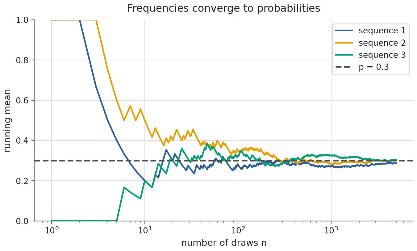

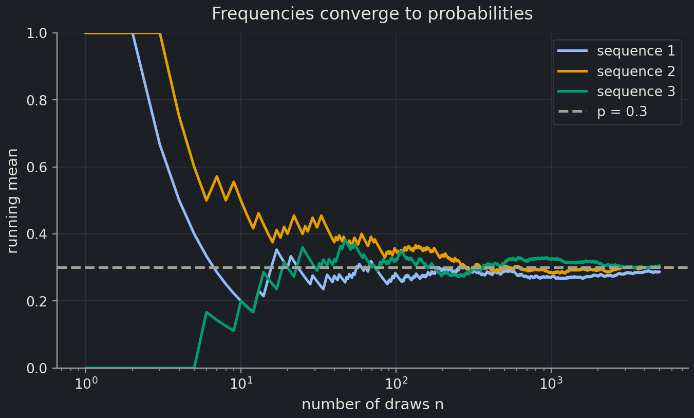
Running mean of Bernoulli draws with p = 0.3 against the number of draws on a logarithmic axis from 1 to 5000, for three independent sequences. All three fluctuate widely for the first few dozen draws and then settle onto the dashed horizontal line at 0.3, with the band of fluctuation narrowing as the number of draws grows.

The law of large numbers says where the average goes. The next theorem says what its fluctuations look like on the way, whatever the distribution of a single draw.

Theorem 12

Central limit theorem

Let \(X_1, X_2, \ldots\) be i.i.d. with mean \(\mu\) and finite variance \(\sigma^2 > 0\). Then for every real \(z\), \[ P\Big( \frac{\bar{X}_n - \mu}{\sigma / \sqrt{n}} \le z \Big) \longrightarrow \Phi(z) \quad \text{as } n \to \infty . \] In words: for large \(n\), \(\bar{X}_n\) is approximately \(N(\mu, \sigma^2 / n)\).

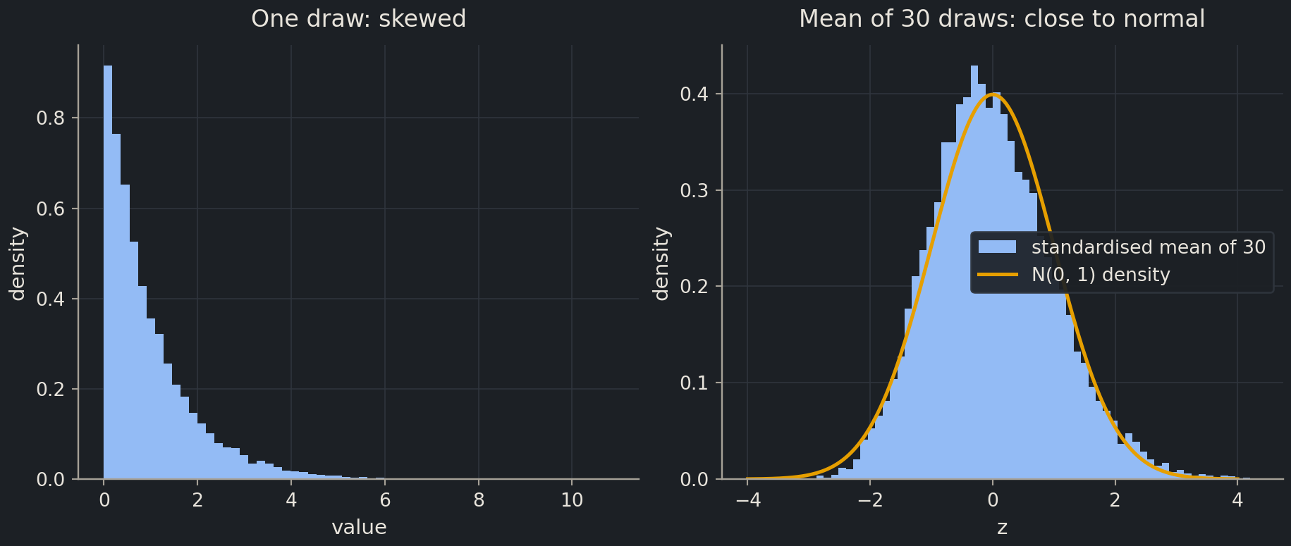
The proof needs more machinery than this appendix builds (characteristic functions) and is in any probability text. The theorem is easy to watch, though: a single draw from an exponential distribution is strongly skewed, but the standardised mean of 30 such draws is already close to the standard normal curve.

draws = rng.exponential(scale=1.0, size=(20_000, 30))
z_means = (draws.mean(axis=1) - 1.0) / (1.0 / np.sqrt(30))  # mean 1 and sd 1 for this distribution
z_grid = np.linspace(-4, 4, 200)

fig, (ax1, ax2) = plt.subplots(1, 2, figsize=(9.5, 4))
ax1.hist(draws[:, 0], bins=60, density=True)
ax1.set(title="One draw: skewed", xlabel="value", ylabel="density")
ax2.hist(z_means, bins=60, density=True, label="standardised mean of 30")
ax2.plot(z_grid, np.exp(-z_grid**2 / 2) / np.sqrt(2 * np.pi), label="N(0, 1) density")
ax2.set(title="Mean of 30 draws: close to normal", xlabel="z", ylabel="density")
ax2.legend()
plt.show()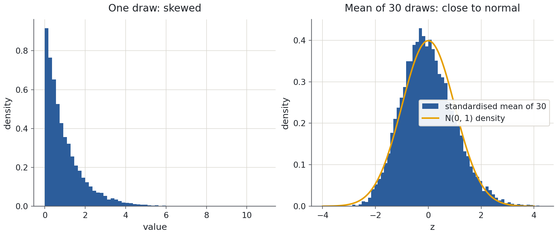

Two histograms side by side. Left: 20,000 single draws from an exponential distribution with mean 1, piled up at zero with a long right tail. Right: the standardised means of 30 draws each, a nearly symmetric bell centred on zero that closely follows the overlaid standard normal density curve.

Together the two theorems are why every number reported from a test set is an estimate with a predictable error bar. The accuracy of a classifier on 226 held-out molecules is the sample mean of 226 Bernoulli variables (“prediction \(i\) was correct”), so its standard deviation is about \(\sqrt{p(1-p)/226}\), roughly 0.03 for \(p\) near 0.8, and by the central limit theorem an approximate 95% interval is the accuracy plus or minus twice that, about \(\pm 0.05\). Two models whose test accuracies differ by one percentage point are not distinguishable by that test set, whatever the leaderboard says. The same reasoning applies to the MAE and the MSE, which are sample means of per-molecule errors (and so to the RMSE, the square root of the MSE), and it is the reason episode 2.4 repeats the split with cross-validation.

Exercise★☆☆

A rarer activity

Repeat the screening calculation with a prevalence of 0.2% instead of 2%, keeping the sensitivity at 90% and the false-positive rate at 5%. What fraction of flagged compounds are now active? What would the false-positive rate have to fall to for that fraction to reach one half?

SolutionShow solution

With \(P(A) = 0.002\): \(P(A \mid F) = 0.9 \times 0.002 / (0.9 \times 0.002 + 0.05 \times 0.998) = 0.0018 / 0.0517 \approx 0.035\), about one flagged compound in thirty. For \(P(A \mid F) = 0.5\) the two terms in the denominator must be equal: the false-positive rate \(r\) must satisfy \(r \times 0.998 = 0.0018\), so \(r \approx 0.0018\), a false-positive rate of 0.18%, nearly thirty times better than before. Prevalence, not assay quality, is the limiting factor.

prev = 0.002
0.9 * prev / (0.9 * prev + 0.05 * (1 - prev)), 0.9 * prev / (1 - prev)

(0.03481624758220503, 0.001803607214428858)

Exercise★☆☆

Actives on a plate

A 96-well plate holds independent compounds, each active with probability 2%. What are the expected number of actives and its standard deviation? What is the probability that the plate has no active at all?

SolutionShow solution

The count is binomial with \(n = 96\) and \(p = 0.02\), so its mean is \(np = 1.92\) and its standard deviation \(\sqrt{np(1-p)} = \sqrt{1.8816} \approx 1.37\). No active means 96 independent failures: \(0.98^{96} \approx 0.144\), so about one plate in seven is empty.

96 * 0.02, (96 * 0.02 * 0.98) ** 0.5, 0.98**96, (plates == 0).mean()

(1.92, 1.3717142559585798, 0.1437815848877014, np.float64(0.14389))

The last number is the fraction of empty plates among the 100,000 simulated above, which agrees.

Exercise★★☆

Variance of a rescaled variable

Prove item 3 of the rules for expectation, variance and covariance: \(\operatorname{Var}(aX + b) = a^2 \operatorname{Var}(X)\). Then say in one sentence why standardising a feature (subtracting its mean, dividing by its standard deviation) gives it variance exactly 1, and why for independent \(X\) and \(Y\) the variance of the difference \(X - Y\) is \(\operatorname{Var}(X) + \operatorname{Var}(Y)\), with a plus sign.

SolutionShow solution

Let \(\mu = \mathbb{E}[X]\). By linearity \(\mathbb{E}[aX + b] = a\mu + b\), so \[ \operatorname{Var}(aX + b) = \mathbb{E}\big[(aX + b - a\mu - b)^2\big] = \mathbb{E}\big[a^2 (X - \mu)^2\big] = a^2\, \mathbb{E}\big[(X - \mu)^2\big] = a^2 \operatorname{Var}(X). \] Standardising is the case \(a = 1/\sigma\), \(b = -\mu/\sigma\), so the variance becomes \(\sigma^2 / \sigma^2 = 1\) and the shift by \(b\) changes nothing. For the difference, \(X - Y = X + (-1)Y\), and \(-Y\) is independent of \(X\) with \(\operatorname{Var}(-Y) = (-1)^2 \operatorname{Var}(Y)\): uncertainties add even when the quantities are subtracted, which is why the difference of two noisy measurements is noisier than either.

Mean, variance and distributions

Used in episode 1.4, episode 1.5 (exploring data) and episode 2.6 (standardisation).

The previous section was about random variables, which are idealised objects. This one is about a list of numbers you actually have, \(x_1, \ldots, x_n\), and the summaries computed from it. The two meet through the law of large numbers: for an i.i.d. sample the quantities below estimate the corresponding expectations.

Definition 26

Sample mean, median and variance

For numbers \(x_1, \ldots, x_n\), the sample mean, sample variance and sample standard deviation are \[ \bar{x} = \frac{1}{n}\sum_{i=1}^{n} x_i, \qquad s^2 = \frac{1}{n - \text{ddof}}\sum_{i=1}^{n} (x_i - \bar{x})^2, \qquad s = \sqrt{s^2}, \] where \(\text{ddof}\) (delta degrees of freedom) is \(0\) or \(1\) by convention, see below. The median is the middle value of the sorted list, or the mean of the two middle values when \(n\) is even.

Theorem 13

What the mean and the median minimise

For numbers \(x_1, \ldots, x_n\):

the sample mean is the unique minimiser of \(c \mapsto \sum_i (x_i - c)^2\);
the median minimises \(c \mapsto \sum_i |x_i - c|\) (when \(n\) is even, every \(c\) between the two middle values does).

ProofShow proof

For item 1, the function \(S(c) = \sum_i (x_i - c)^2\) has derivative \(S'(c) = -2 \sum_i (x_i - c) = -2(n\bar{x} - nc)\), which vanishes only at \(c = \bar{x}\), and \(S''(c) = 2n > 0\), so that point is the minimum. For item 2, between consecutive data points the function \(\sum_i |x_i - c|\) is linear in \(c\) with slope (number of \(x_i\) below \(c\)) minus (number above \(c\)). The slope is negative while fewer than half the points lie below \(c\) and positive once more than half do, so the function decreases until \(c\) reaches the median and increases afterwards.

The theorem explains two things used all over the course. The mean is what you get by minimising a squared error, which is why the mean is the natural baseline for a model trained with mean squared error (MSE); and the median is what you get by minimising an absolute error, which is why it is robust to a few extreme values (moving one far-away point changes the slope count by one, not the value by a lot).

Which denominator?

Proposition 14

The n − 1 denominator

Let \(X_1, \ldots, X_n\) be i.i.d. with variance \(\sigma^2\), let \(\bar{X}\) be their mean, and let \(S^2 = \frac{1}{n - 1}\sum_i (X_i - \bar{X})^2\). Then \(S^2\) is unbiased, \(\mathbb{E}[S^2] = \sigma^2\), whereas the version with \(n\) in the denominator has expectation \(\frac{n-1}{n}\sigma^2\), slightly too small.

ProofShow proof

Write \(\mu\) for the common mean. Adding and subtracting \(\mu\) inside the square and expanding gives the identity \(\sum_i (X_i - \bar{X})^2 = \sum_i (X_i - \mu)^2 - n(\bar{X} - \mu)^2\) (the cross term is \(-2(\bar{X} - \mu)\sum_i(X_i - \mu) = -2n(\bar{X} - \mu)^2\)). Taking expectations, \(\mathbb{E}[(X_i - \mu)^2] = \sigma^2\) for each \(i\) and \(\mathbb{E}[(\bar{X} - \mu)^2] = \operatorname{Var}(\bar{X}) = \sigma^2 / n\), so the expected sum is \(n\sigma^2 - \sigma^2 = (n - 1)\sigma^2\). Dividing by \(n - 1\) gives \(\sigma^2\); dividing by \(n\) gives \(\frac{n-1}{n}\sigma^2\).

Libraries disagree about the default, so check rather than assume: draw twenty values from the seeded random number generator and ask NumPy and pandas for the standard deviation.

sample = rng.normal(loc=10, scale=2, size=20)
np.std(sample), pd.Series(sample).std()

(np.float64(1.6927296219387793), np.float64(1.7367039480424746))

np.std(sample, ddof=1)  # now equal to the pandas value

np.float64(1.7367039480424746)

NumPy uses ddof=0 and pandas uses ddof=1. scikit-learn’s StandardScaler uses ddof=0, like NumPy. With a few hundred samples the difference is well under 1%; what matters is knowing which one a number is before you compare it with another.

Standardisation: z-scores

Definition 27

z-score

The z-score of a value \(x_i\) in a list with mean \(\bar{x}\) and standard deviation \(s\) is \(z_i = (x_i - \bar{x}) / s\). The list \(z_1, \ldots, z_n\) has mean \(0\) and standard deviation \(1\) (with the same \(\text{ddof}\) used to compute \(s\)).

A z-score says how many standard deviations a value sits above (positive) or below (negative) the typical value, whatever the original units; that is what makes features comparable in the distance section above.

mass = penguins["body_mass_g"]
z = (mass - mass.mean()) / mass.std()
z.describe().round(2)

count    333.00
mean      -0.00
std        1.00
min       -1.87
25%       -0.82
50%       -0.20
75%        0.71
max        2.60
Name: body_mass_g, dtype: float64

Biologist's corner

Expression heatmaps are almost always z-scored gene by gene before plotting. Each row is centred on that gene’s own mean and scaled by its own spread, so the colour says “above or below this gene’s usual level in this sample”, not “high or low counts”. Without that step the few highly expressed genes would set the colour scale and everything else would look flat.

The normal distribution in data

Many measurements, and most noise, pile up around a central value in a symmetric bell shape: the normal distribution of the previous section, fixed entirely by its mean \(\mu\) and standard deviation \(\sigma\). The central limit theorem is one reason: a quantity built from many small independent contributions tends to be approximately normal.

Proposition 15

The 68–95–99.7 rule

If \(X \sim N(\mu, \sigma^2)\) then, to three decimal places, \[ P(|X - \mu| \le \sigma) = 0.683, \qquad P(|X - \mu| \le 2\sigma) = 0.954, \qquad P(|X - \mu| \le 3\sigma) = 0.997 . \]

ProofShow proof

By the standardisation in the proposition on the four distributions, \(P(|X - \mu| \le k\sigma) = \Phi(k) - \Phi(-k)\), and the values are those computed with math.erf in the probability section: 0.6827, 0.9545 and 0.9973.

A large random sample agrees, to within sampling error (about \(\pm 0.003\) for 100,000 draws):

big = rng.normal(loc=0, scale=1, size=100_000)
[np.mean(np.abs(big) < k).round(3) for k in (1, 2, 3)]

[np.float64(0.682), np.float64(0.953), np.float64(0.997)]

Compare these with the law of large numbers’ bound \(\sigma^2 / (n\varepsilon^2)\), which for \(n = 1\) and \(\varepsilon = 2\sigma\) only promises \(P(|X - \mu| \ge 2\sigma) \le 1/4\). Chebyshev’s inequality holds for every distribution and is correspondingly loose; the normal distribution is much more concentrated than the worst case.

Real data is rarely this tidy. Here is the histogram of penguin body mass with the normal curve of the same mean and standard deviation drawn over it.

mu, sigma = mass.mean(), mass.std()
grid = np.linspace(2000, 7000, 300)
normal_pdf = np.exp(-0.5 * ((grid - mu) / sigma) ** 2) / (sigma * np.sqrt(2 * np.pi))

fig, ax = plt.subplots()
ax.hist(mass, bins=25, density=True, alpha=0.6, label="penguins")
ax.plot(grid, normal_pdf, label="normal curve, same mean and sd")
ax.set(xlabel="body mass (g)", ylabel="density", title="Body mass of 333 penguins")
ax.legend()
plt.show()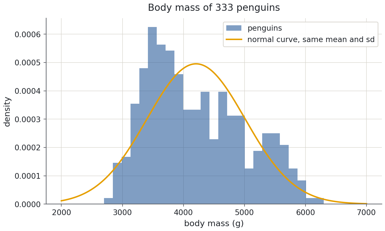

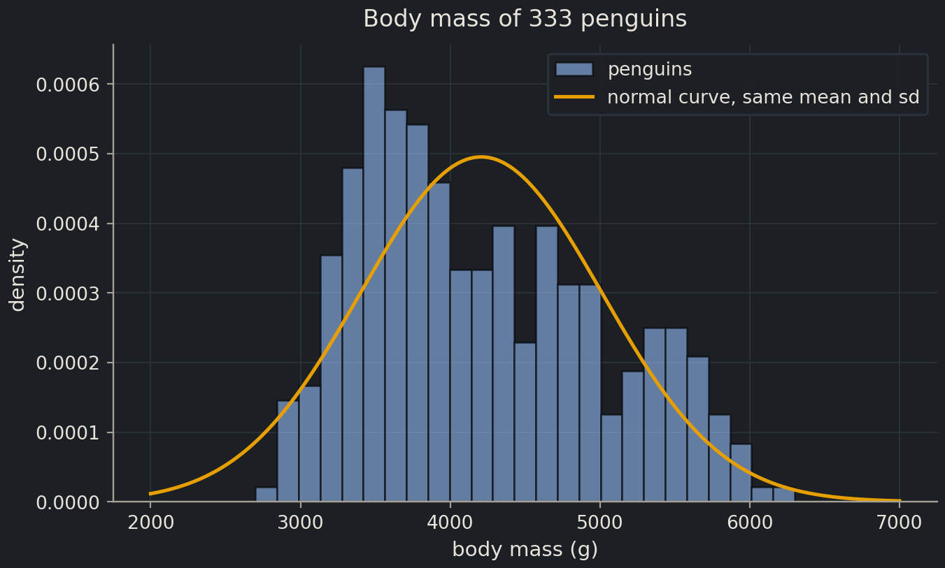
A histogram of penguin body mass in grams, from about 2700 to 6300 g, with a smooth bell-shaped normal curve overlaid. The histogram is not a single bell: a tall hump around 3500 g and a lower, broader hump around 5000 g, so the right tail is heavier than the curve predicts.

The curve is a poor summary. The data have two humps, Adelie and Chinstrap penguins around 3500 g and the larger Gentoo around 5000 g, so the right tail is heavier than a single bell predicts. With this skew the mean (about 4207 g) sits above the median (4050 g): the mean is pulled by every value in the tail, while the median depends only on the order of the values.

with_typo = np.append(mass.to_numpy(), 42070.0)  # one mass entered with an extra zero
(mass.mean(), with_typo.mean()), (mass.median(), np.median(with_typo))

((np.float64(4207.057057057057), np.float64(4320.419161676647)),
 (np.float64(4050.0), np.float64(4050.0)))

The mean jumps by over 100 g; the median moves by nothing worth mentioning, as the theorem on what the median minimises predicts. When a quantity is skewed or may contain outliers, report the median alongside the mean, or fix the skew with a logarithm (next section).

Correlation

Definition 28

Pearson correlation

For paired numbers \((x_1, y_1), \ldots, (x_n, y_n)\) with z-scores \(z^x_i\) and \(z^y_i\) (computed with \(\text{ddof} = 0\)), the Pearson correlation is \[ r = \frac{1}{n} \sum_{i=1}^{n} z^x_i\, z^y_i = \frac{\sum_i (x_i - \bar{x})(y_i - \bar{y})}{\sqrt{\sum_i (x_i - \bar{x})^2}\, \sqrt{\sum_i (y_i - \bar{y})^2}} . \] It is the sample version of the correlation \(\rho\) of two random variables.

Proposition 16

Bounds on the correlation

\(-1 \le r \le 1\), and \(r = \pm 1\) exactly when the points lie on a straight line with positive (respectively negative) slope.

ProofShow proof

The second form of \(r\) is the cosine similarity of the two centred vectors \(u = (x_i - \bar{x})_i\) and \(v = (y_i - \bar{y})_i\), so the Cauchy–Schwarz inequality gives \(|r| \le 1\), with equality exactly when \(v = \lambda u\) for some scalar \(\lambda\), that is when \(y_i - \bar{y} = \lambda (x_i - \bar{x})\) for every \(i\): a straight line of slope \(\lambda\), whose sign is the sign of \(r\).

Near \(1\) the two variables rise together along a line, near \(-1\) one falls as the other rises, near \(0\) there is no linear relationship. Flipper length and body mass in penguins are strongly correlated.

np.corrcoef(penguins["flipper_length_mm"], penguins["body_mass_g"])[0, 1].round(3)

np.float64(0.873)

Two cautions. correlation coefficient measures straight-line association only: a perfect U-shaped relationship scores close to zero, exactly like the \(Y = X^2\) example of the probability section. And it can reverse when groups are mixed: bill length and bill depth are negatively correlated across all penguins but positively correlated within each species, because the species differ in both. Always look at the scatter plot, coloured by group, before trusting a single \(r\).

Exercise★☆☆

Statistics by hand

For the values 2, 4, 4, 4, 5, 5, 7, 9, compute the mean, the median, the population variance and standard deviation (ddof=0), and the sample standard deviation (ddof=1). Check with NumPy and pandas.

SolutionShow solution

Mean \(= 40 / 8 = 5\). Median: the sorted middle pair is 4 and 5, so \(4.5\). Squared deviations: \(9, 1, 1, 1, 0, 0, 4, 16\), summing to \(32\). Population variance \(= 32/8 = 4\), standard deviation \(2\). Sample variance \(= 32/7 \approx 4.57\), standard deviation \(\approx 2.14\).

vals = np.array([2, 4, 4, 4, 5, 5, 7, 9])
vals.mean(), np.median(vals), vals.var(), vals.std(), pd.Series(vals).std()

(np.float64(5.0),
 np.float64(4.5),
 np.float64(4.0),
 np.float64(2.0),
 np.float64(2.138089935299395))

vals.std() gives 2 and pd.Series(vals).std() gives 2.14: the same data, two defaults.

Logarithms

Used in episode 1.5 (the solubility target) and throughout Part II.

Definition 29

Logarithm

For a base \(b > 0\), \(b \ne 1\), and \(x > 0\), the logarithm \(\log_b x\) is the unique real number \(y\) with \(b^y = x\). The two bases in everyday use are \(10\), written \(\log_{10}\), and Euler’s number \(e \approx 2.718\), whose logarithm is the natural logarithm \(\ln\). Logarithms of zero or of negative numbers are not defined.

Proposition 17

Laws of logarithms

For \(a, c > 0\), any real \(k\), and any valid base:

\(\log(ac) = \log a + \log c\) and \(\log(a / c) = \log a - \log c\);
\(\log a^k = k \log a\);
for a base greater than 1 (in particular \(10\) and \(e\)), \(\log\) is strictly increasing, so it preserves order: \(a < c\) if and only if \(\log a < \log c\);
change of base: \(\log_{10} x = \ln x / \ln 10 \approx \ln x / 2.303\).

ProofShow proof

Write \(a = b^{u}\) and \(c = b^{v}\) for the base \(b\), so that \(u = \log a\) and \(v = \log c\). Then \(ac = b^{u + v}\), \(a/c = b^{u - v}\) and \(a^k = b^{ku}\), which by the definition give items 1 and 2. Item 3 holds because \(y \mapsto b^y\) is strictly increasing when \(b > 1\) (for \(0 < b < 1\) it is strictly decreasing, and so is \(\log_b\)). For item 4, \(x = e^{\ln x} = 10^{\ln x / \ln 10}\) since \(10 = e^{\ln 10}\).

Items 3 and 4 together say that \(\log_{10}\) and \(\ln\) never disagree about order, only about scale; item 4 gives the scale factor.

np.log10([1, 10, 100, 1000, 0.001])

array([ 0.,  1.,  2.,  3., -3.])

np.log(10.0), np.log10(10.0)

(np.float64(2.302585092994046), np.float64(1.0))

Common mistake

np.log is the natural logarithm

np.log(100) is about 4.6, not 2. If you want powers of ten, write np.log10. The same trap exists in pandas, R and most calculators’ LN button. NumPy returns -inf or nan (and a warning) for the logarithm of zero or of a negative number, which the definition says does not exist.

a_val, c_val = 200.0, 50.0
np.log10(a_val * c_val), np.log10(a_val) + np.log10(c_val)

(np.float64(4.0), np.float64(4.0))

Why scientists work in logs

Measured solubilities in the ESOL dataset run from about \(10^{-11.6}\) to \(10^{1.6}\) mol/L: thirteen orders of magnitude. On a linear axis the soluble handful would fill the plot and the rest would be a smear at zero. On a log axis each unit is a factor of ten and the whole range is visible. More importantly for modelling, errors and effects in chemistry and biology are usually multiplicative (“twice as soluble”, “a three-fold increase in expression”), and by item 1 a logarithm turns multiplicative into additive, which is what a linear model and a squared-error loss assume. That is the point of a log transform.

Chemist's corner

You already think in logs: pH \(= -\log_{10}[\mathrm{H^+}]\), so pH 3 to pH 6 is a thousand-fold drop in hydrogen-ion concentration, and p\(K_a\), logP and logS work the same way. An ESOL model with an RMSE of 0.5 logS units is therefore typically wrong by a factor of \(10^{0.5} \approx 3\) in solubility. Keep that conversion in your head whenever a chapter reports an error in log units.

Geometric versus arithmetic mean

Definition 30

Geometric mean

The geometric mean of positive numbers \(x_1, \ldots, x_n\) is \(\big(\prod_{i=1}^{n} x_i\big)^{1/n}\). By the laws of logarithms its logarithm is the arithmetic mean of the logarithms, \(\log \text{GM} = \frac{1}{n}\sum_i \log x_i\).

Theorem 14

Arithmetic–geometric mean inequality

For positive \(x_1, \ldots, x_n\), \[ \Big(\prod_{i=1}^{n} x_i\Big)^{1/n} \le \frac{1}{n} \sum_{i=1}^{n} x_i , \] with equality if and only if all the \(x_i\) are equal.

ProofShow proof

For \(n = 2\): \((\sqrt{x_1} - \sqrt{x_2})^2 \ge 0\) expands to \(x_1 + x_2 \ge 2\sqrt{x_1 x_2}\), with equality only when \(x_1 = x_2\). In general, \(\ln\) is strictly concave (its second derivative \(-1/x^2\) is negative), and Jensen’s inequality for a strictly concave function, which we use without proof, gives \(\ln\big(\frac{1}{n}\sum_i x_i\big) \ge \frac{1}{n}\sum_i \ln x_i = \ln \text{GM}\), with equality only when all the \(x_i\) are equal. Taking exponentials, which preserve order, finishes the proof.

For quantities spanning orders of magnitude the arithmetic mean is dominated by the largest values, and the theorem says it is always at least the geometric mean. The geometric mean is the honest “typical value” for concentrations, fold-changes and rate constants.

conc = np.array([1e-6, 1e-5, 1e-4, 1e-3, 1e-2])  # mol/L
conc.mean(), 10 ** np.mean(np.log10(conc))

(np.float64(0.0022221999999999997), np.float64(0.0001))

The arithmetic mean, \(2.2 \times 10^{-3}\), is larger than four of the five values; the geometric mean, \(10^{-4}\), is the middle one.

Undoing a log

To get back from a log value to the quantity, raise the base to that power: 10 ** x for \(\log_{10}\), np.exp(x) for \(\ln\). A predicted logS of \(-3.5\) is a solubility of \(10^{-3.5} \approx 3.2 \times 10^{-4}\) mol/L.

logS = -3.5
10**logS

0.00031622776601683794

Making a skewed quantity symmetric

Definition 31

Log-normal distribution

A positive random variable \(X\) is log-normal if \(\ln X\) is normal. Its raw values are typically right-skewed, piling up at the low end with a long right tail; its logarithms form a symmetric bell.

skewed = rng.lognormal(mean=0, sigma=0.8, size=2000)

fig, (ax1, ax2) = plt.subplots(1, 2, figsize=(9.5, 4))
for ax, values, label in [(ax1, skewed, "raw value"), (ax2, np.log10(skewed), "log10(value)")]:
    ax.hist(values, bins=40)
    ax.axvline(values.mean(), linestyle="--", color="0.3", label="mean")
    ax.axvline(np.median(values), linestyle=":", color="0.3", label="median")
    ax.set(xlabel=label, ylabel="count")
ax1.set(title="Raw: skewed")
ax2.set(title="After log10: symmetric")
ax1.legend()
plt.show()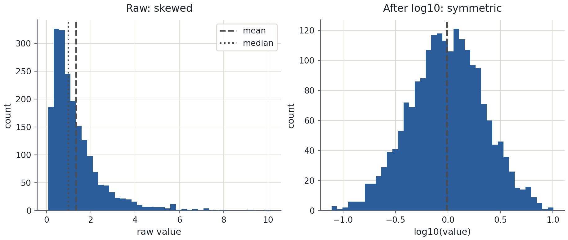

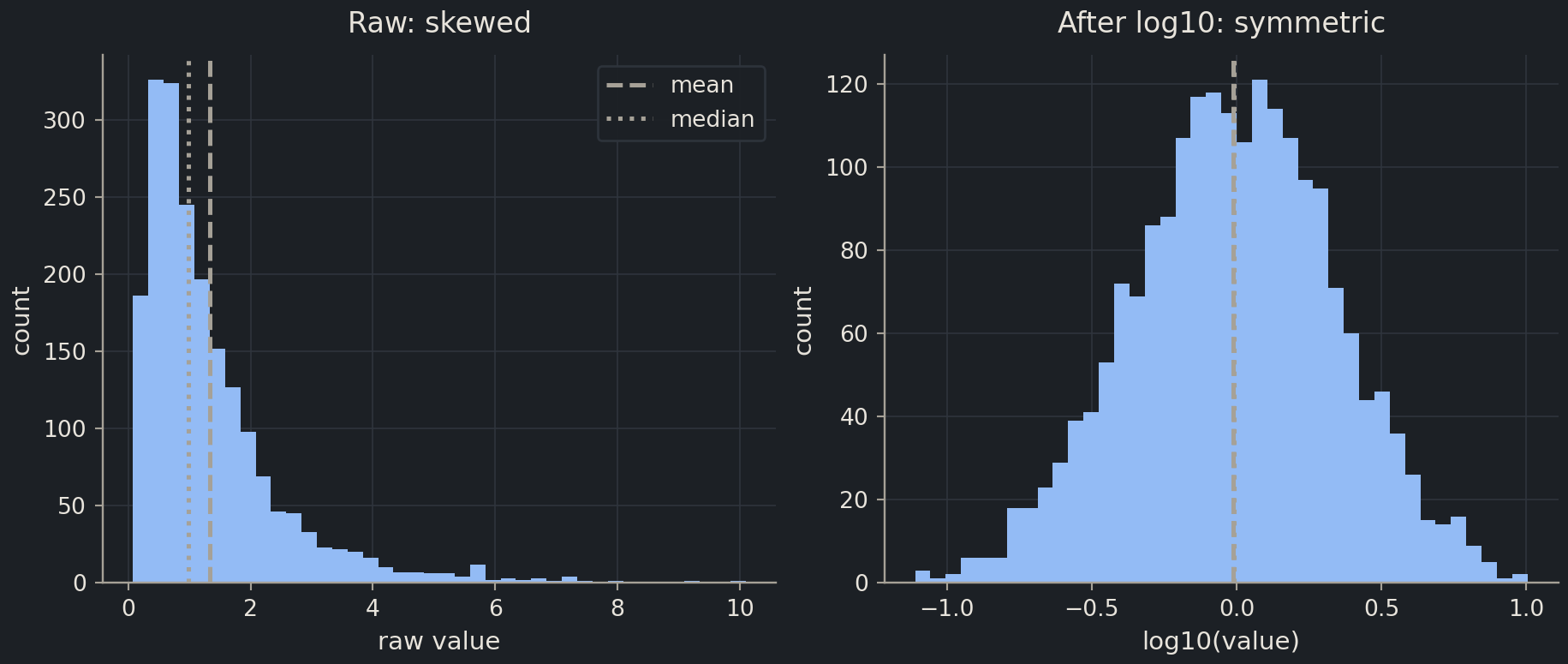
Two histograms side by side. Left: a log-normal sample on its raw scale, strongly right-skewed with most values below 3 and a thin tail stretching past 10; the mean (dashed line) sits to the right of the median (dotted line). Right: the base-10 logarithm of the same values, a symmetric bell centred on zero, with the mean and median lines almost on top of each other.

On the raw scale the mean is pulled far to the right of the median by the tail. The median of a log-normal variable is its geometric mean, so the arithmetic–geometric inequality says the mean must sit to its right. After the log transform the two coincide, the standard deviation means what the 68–95–99.7 rule says it means, and a squared-error loss no longer spends all its effort on the few largest values. This is why the solubility target is modelled as logS and never as mol/L.

Exercise★☆☆

Factors of ten

Compound A has logS \(= -2\) and compound B has logS \(= -5\). How many times more soluble is A? What is the solubility of B in mol/L? And what is np.log(1000), roughly: 3, or something else?

SolutionShow solution

The difference in logS is 3, so by the quotient law A is \(10^3 = 1000\) times more soluble. B’s solubility is \(10^{-5}\) mol/L (10 µmol/L). np.log(1000) is the natural log, about 6.9; np.log10(1000) is 3, and the ratio of the two is \(\ln 10 \approx 2.303\) as the change-of-base law says.

10 ** (-2 - (-5)), 10**-5, np.log(1000), np.log10(1000)

(1000, 1e-05, np.float64(6.907755278982137), np.float64(3.0))

Notation

Vectors and vector spaces

Linear combinations, independence and bases

Matrices and linear maps

Products

Linear maps

Column space, null space and rank

Identity, inverse, and why we solve

Inner products, norms and distances

Norms in general

Distance between two samples

Derivatives and gradients

A loss curve and its tangent

Several parameters: partial derivatives and the gradient

Least squares

Probability

Probability spaces

Random variables and their distributions

Expectation, variance and covariance

Four distributions

Averages of many samples

Mean, variance and distributions

Which denominator?

Standardisation: z-scores

The normal distribution in data

Correlation

Logarithms

Why scientists work in logs

Geometric versus arithmetic mean

Undoing a log

Making a skewed quantity symmetric

Identity, inverse, and why we `solve`