Why should I draw a picture before I compute a statistic?
What are a Figure and an Axes, and why does the course always write fig, ax = plt.subplots()?
Which plot do I use for one variable, two variables, or a whole table of them?
What you will be able to do
Build a scatter plot with the matplotlib object-oriented API and label it with units.
Compare distributions across groups with sns.histplot, sns.boxplot and sns.violinplot.
Survey a whole table at once with sns.pairplot and a correlation heatmap.
Choose colour-blind-safe palettes and arrange several panels with plt.subplots(1, 2).
Save a figure at publication resolution with fig.savefig.
In episode 1.3 you computed, per species, the mean flipper length and body mass of 344 penguins. Two numbers per species. Now imagine a reviewer asks: “Are the three species really separate, or do they overlap? Is anything odd in the data?” Those questions are about shape, and shape is what a picture shows and a summary statistic hides. The same reviewer will ask the same question of every solubility, toxicity or expression dataset you meet later in this course, so this episode builds the habit of looking before computing.
Two libraries do almost all of the work. matplotlib draws: it owns the canvas, the axes, the text. seaborn sits on top of it and knows about DataFramesDataFramepandas’ table type: labelled rows and columns, each column with its own data type.: give it a table and a column name, and it draws a statistical plot with sensible defaults. You will use both in every later chapter.
Anatomy of a matplotlib figure
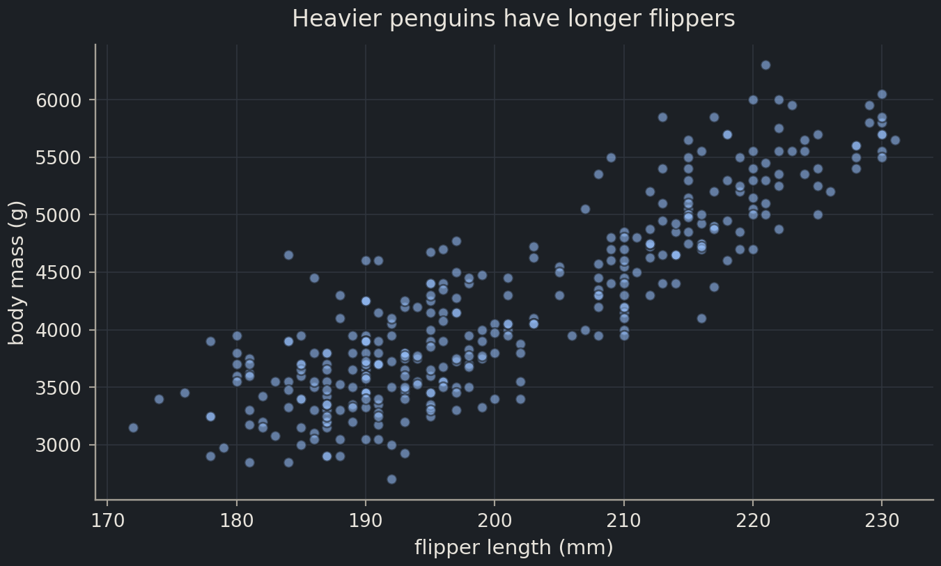
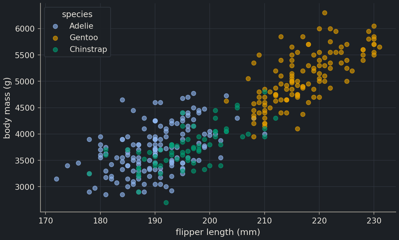
Load the penguins and the two libraries. The hidden setup cell at the top of each episode applies the course’s plotting style, so your figures will look like these if you copy the code.
import matplotlib.pyplot as pltimport pandas as pdimport seaborn as snspenguins = pd.read_csv("data/penguins.csv")penguins.head(3)
index
species
island
bill_length_mm
bill_depth_mm
flipper_length_mm
body_mass_g
sex
year
0
Adelie
Torgersen
39.1
18.7
181.0
3750.0
male
2007
1
Adelie
Torgersen
39.5
17.4
186.0
3800.0
female
2007
2
Adelie
Torgersen
40.3
18.0
195.0
3250.0
female
2007
Every matplotlib picture is built from two objects:
a Figure, the page or window that everything is drawn on;
one or more Axes, a plotting area with an x axis and a y axis. (One Axes, several Axes. It is matplotlib’s word for a panel, not the plural of “axis”.)
plt.subplots() creates both and hands them back as a pair. From then on, you draw by calling methods on the Axes.
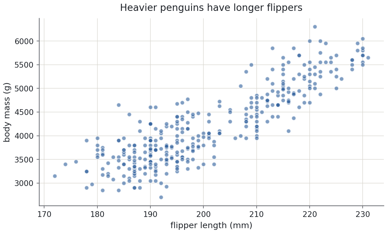
fig, ax = plt.subplots()ax.scatter(penguins["flipper_length_mm"], penguins["body_mass_g"], alpha=0.6)ax.set( xlabel="flipper length (mm)", ylabel="body mass (g)", title="Heavier penguins have longer flippers",)plt.show()
Three things in that cell matter more than they look:
ax.scatter(x, y) draws a scatter plotscatter plotOne point per sample, placed by two numeric variables; the plot for relationships.: one marker per row. The two missing-measurement rows you found in episode 1.3 are silently skipped.
ax.set(...) sets several properties at once. The labels carry units. A plot without units is a sketch, not a figure.
plt.show() ends the cell. In a notebook it displays the figure; in a script it opens a window.
alpha=0.6 makes the markers slightly transparent, so places where many points overlap appear darker. We return to that below.
For programmers
matplotlib has two interfaces. The stateful one, plt.plot(...), plt.xlabel(...), acts on whatever matplotlib considers the “current” figure and axes, a hidden global. It is fine for a two-line sketch at a prompt. The object-oriented one, used throughout this course, names the objects explicitly: fig and ax are ordinary variables you pass to functions, store in lists and return from helpers. With several panels the stateful style becomes a guessing game about which panel plt.xlabel will hit; the OO style never has that ambiguity. Every seaborn function that draws on one panel accepts ax=, so the two libraries mix cleanly.
Common mistake
State that leaks between cells
plt.xlabel("mass") labels the current Axes. If an earlier cell left a figure open, or you created two panels with plt.subplots(1, 2), the current Axes is whichever one matplotlib touched last, usually the right-hand panel. The label lands in the wrong place and nothing warns you. Writing ax.set(xlabel=...) on the Axes you mean removes the guesswork, which is why the course never uses plt.xlabel.
Colour by group
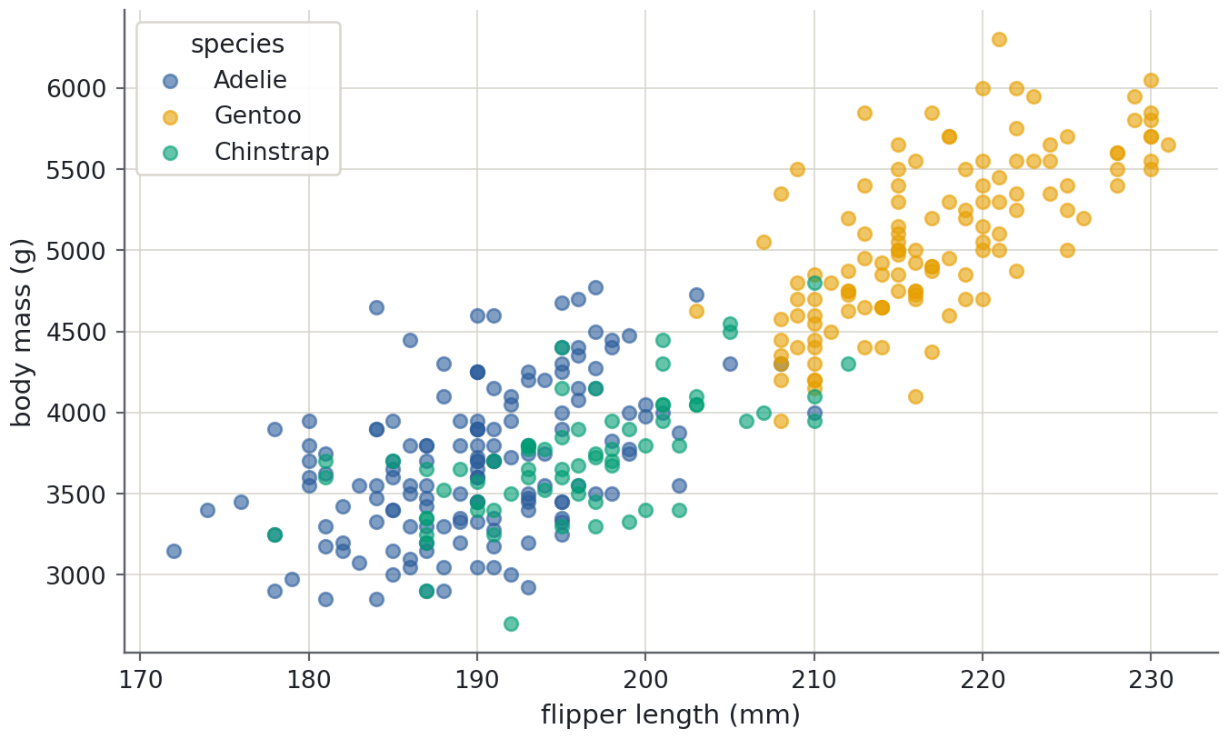
The scatter plot shows two clusters, and you already know there are three species. The first way to colour by group is a loop: draw each species separately, give each call a label, then ask for a legend. Reuse an explicit order and palette so each species keeps the same colour in later plots.
Predict before you run
Before you run the next cell: which species will sit at the top right (long flippers, heavy)? Gentoo, the largest species in the table of means from episode 1.3? Write down your guess and whether the other two will be separable.
species_order = ["Adelie", "Gentoo", "Chinstrap"]species_palette =dict(zip(species_order, sns.color_palette(n_colors=3)))fig, ax = plt.subplots()for species in species_order: group = penguins[penguins["species"] == species] ax.scatter( group["flipper_length_mm"], group["body_mass_g"], color=species_palette[species], alpha=0.6, label=species, )ax.set(xlabel="flipper length (mm)", ylabel="body mass (g)")ax.legend(title="species")plt.show()
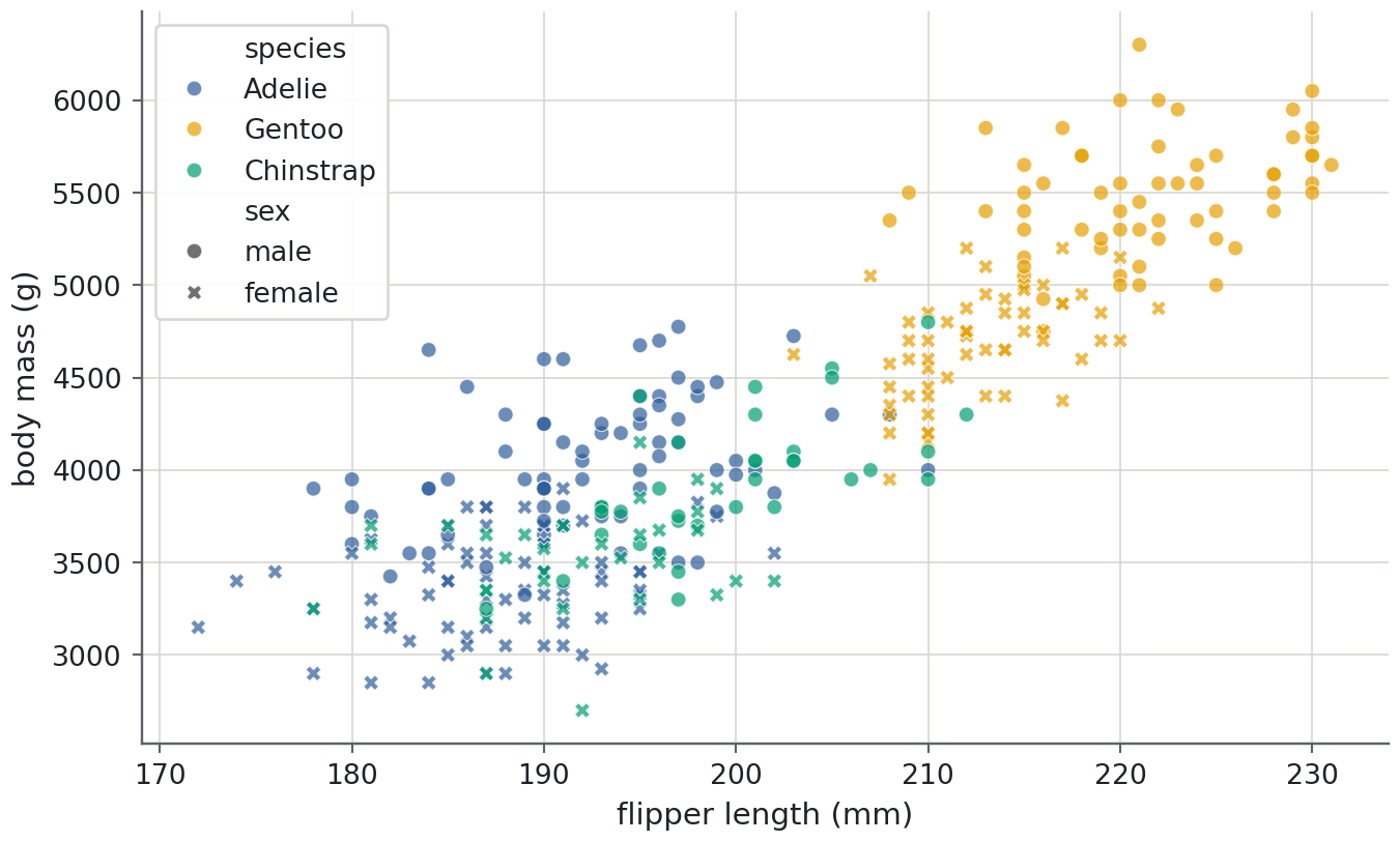
Gentoo penguins are indeed the separate cluster. Adelie and Chinstrap overlap almost completely in these two measurements, something a table of means (3,701 g versus 3,733 g) hinted at but could not show.
The loop works, but seaborn does the same in one call. hue colours by a categorical datacategorical dataA column whose values come from a fixed set of categories, such as species or island. column; style changes the marker shape by another one.
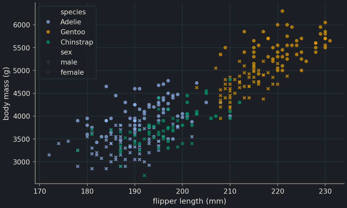
Two encodings on one plot is about the limit before a figure becomes a puzzle. Here it pays off: within each species, males are heavier and longer-flippered than females, so part of the spread inside each cluster is sex, not noise. The penguins with missing sex are left out of the plot without comment, which is one more reason to check isna() before you draw.
One variable: histograms and density curves
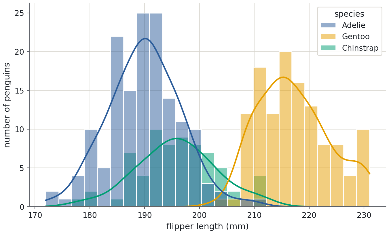
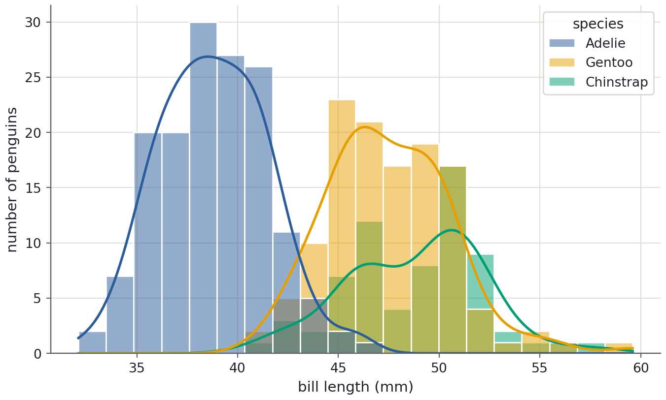
A scatter plot needs two variables. To see the distribution of one, bin it and count: a histogramhistogramBars counting how many values fall into each interval (bin) of a variable.. sns.histplot does the binning, and kde=True overlays a kernel density estimatekernel density estimate (KDE)A smoothed version of a histogram that estimates the probability density., a smoothed curve that shows the shape without the staircase of the bins. hue splits the histogram by group, exactly as in the scatter plot.
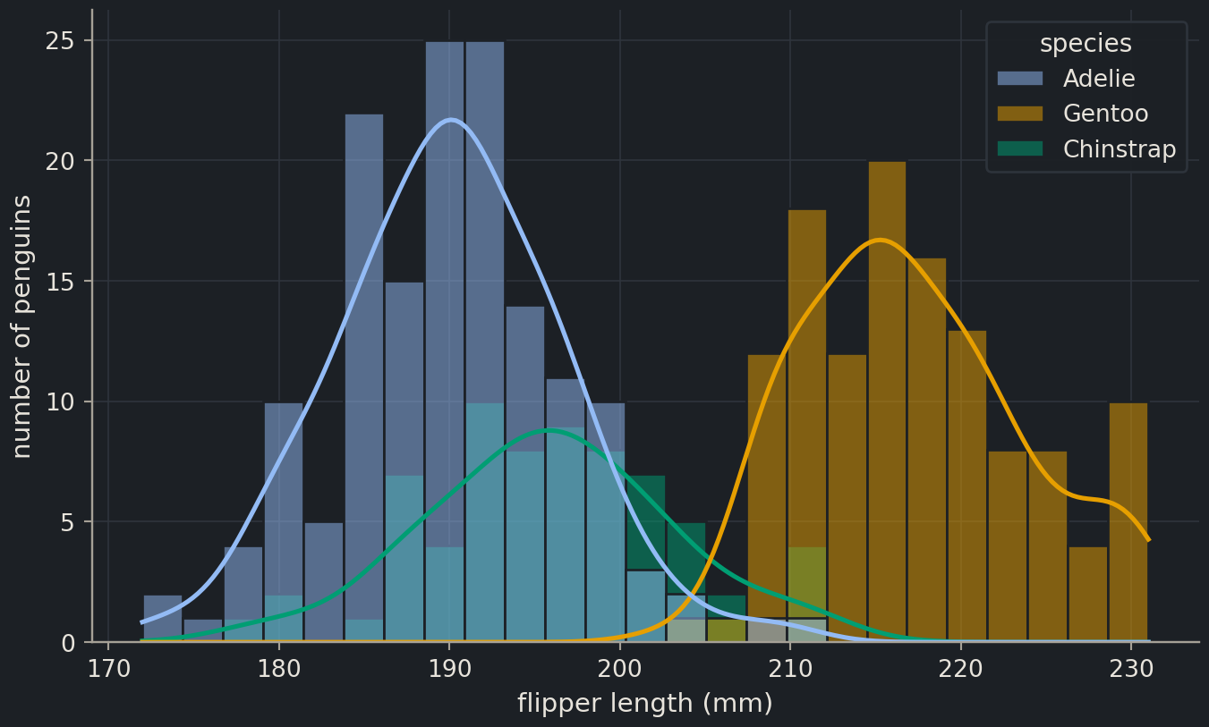
The density curves make the comparison easy to read: three roughly bell-shaped distributions, with Gentoo clearly shifted right. Two cautions. The curve is a smoothed estimate, so with a few dozen points it can invent bumps that are not there; and the number of bins changes how a histogram looks. Try bins=10 and bins=50 and see how much your impression changes, then report the one that is honest rather than the one that is pretty.
One variable per group: box plots and violins
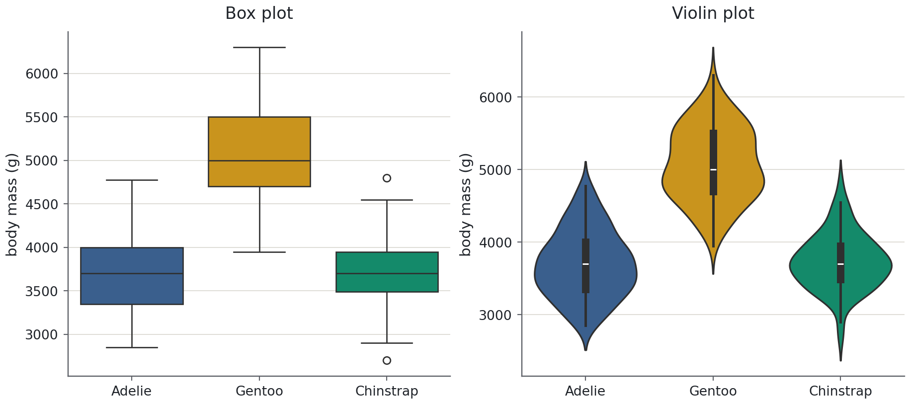
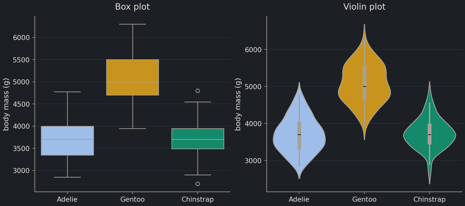
When you have several groups and one measurement, overlapping histograms get crowded. A box plotbox plotA summary of a distribution: median, quartiles and outliers, good for comparing groups. summarises each group as a box from the first to the third quartile with a line at the median, whiskers that reach the most extreme points within 1.5 box-lengths, and individual markers for anything beyond them. A violin plot replaces the box with a mirrored density curve, so you see the shape as well as the quartiles. Draw them side by side with plt.subplots(1, 2), which returns one Figure and an array of two Axes.
Read the box plot for the numbers: the Gentoo median is about 1,300 g above the other two, and its box does not overlap theirs. Read the violin for the shape: the Gentoo violin bulges twice, around 4,700 g and 5,500 g, which is the female and male groups you saw in the scatter plot. A box plot would never have told you that.
(hue="species" together with legend=False is how seaborn 0.13 colours each box by its own category without adding a redundant legend.)
Note
Which plot, when
You want to see
Use
the shape of one variable
histplot (add kde=True with more than about 50 points)
one variable across a few groups
boxplot for the summary, violinplot for the shape, both if space allows
how two variables relate
scatterplot (with hue for a third, categorical variable)
a trend over an ordered axis (time, dose)
ax.plot with lines joining the points
every pair of columns at once
pairplot
the strength of every pairwise relationship
a correlation heatmap
Many variables at once
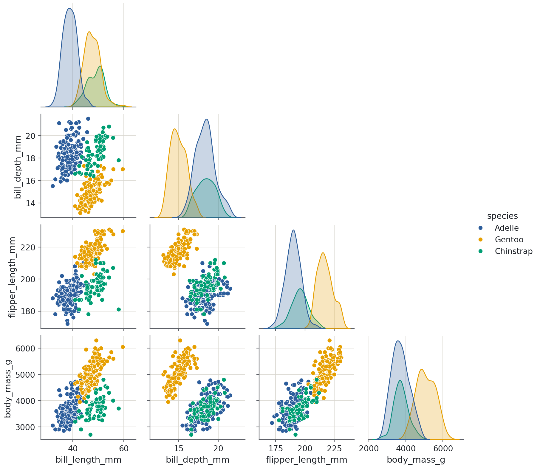
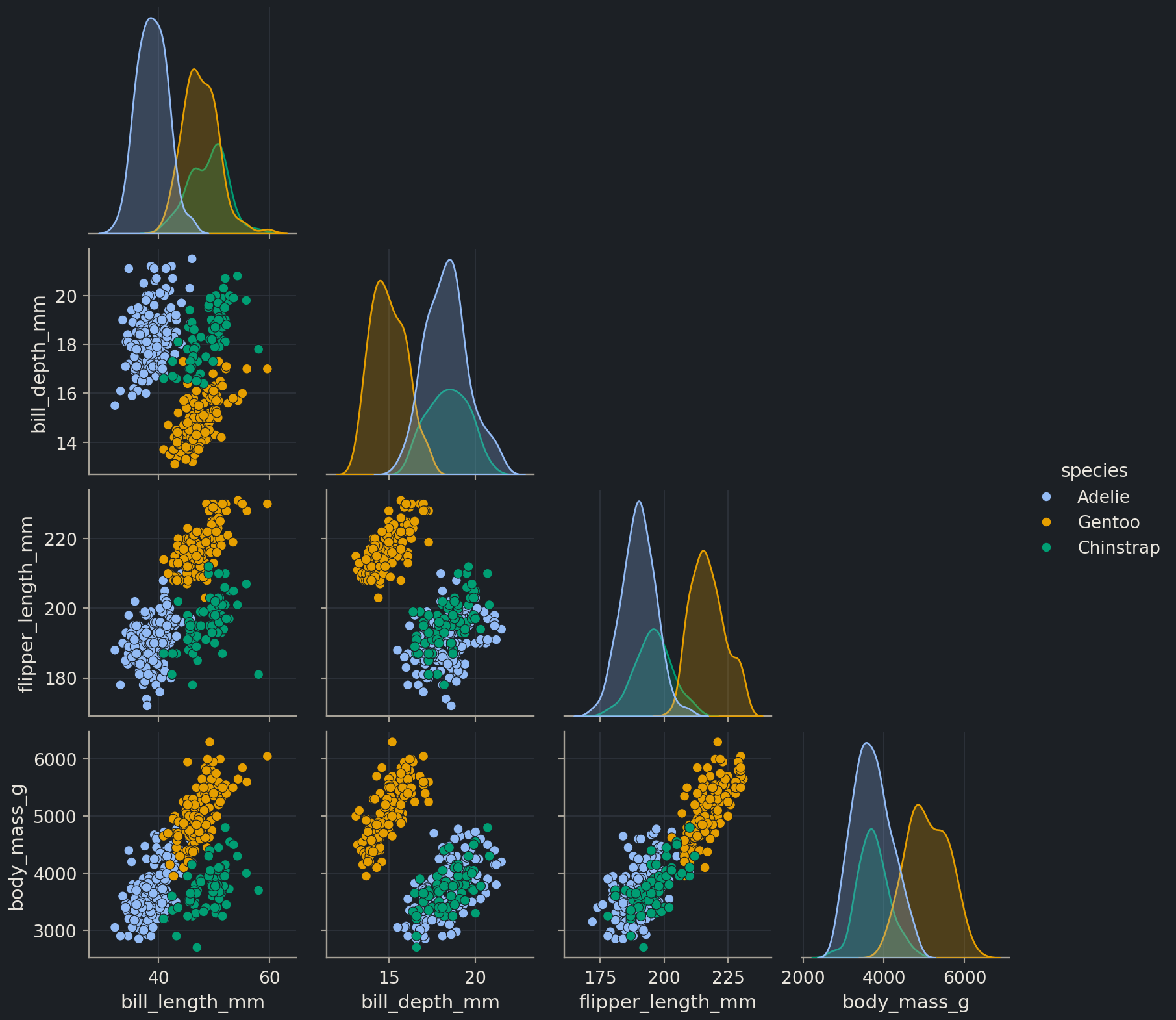
With four measurements you could draw six scatter plots by hand. sns.pairplot draws all of them in a grid, with each variable’s distribution on the diagonal. It is a figure-level function: it creates its own Figure and arranges the panels, so you do not call plt.subplots() first, and you call it alone in a cell. corner=True drops the mirror-image upper half.
Look along the bottom row and down the first column. Flipper length and body mass separate Gentoo from the rest; bill length is the measurement that separates Adelie from Chinstrap. That is exactly the kind of observation that decides which features go into a classifier in Chapter 2, and you got it from one picture.
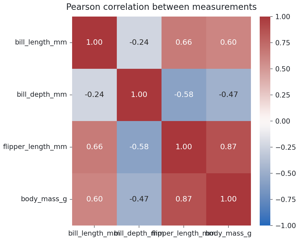
A pairplot shows the relationships; a correlation coefficientcorrelation coefficientA number between −1 and 1 measuring how linearly two variables move together. matrix puts a number on each. The Pearson correlation runs from −1 (one variable falls exactly as the other rises) through 0 (no linear relationship) to +1. df.corr() computes it for every pair of numeric columns, and sns.heatmap colours the resulting table. Drop year first: it is a number, but the correlation between a measurement and the year it was taken is not something you want in the picture.
The strongest pair is flipper length and body mass (0.87), which you already saw as the tight band in the first scatter plot. The surprise is bill depth: it is negatively correlated with flipper length and body mass. Scroll back to the pairplot before you believe it. Within each species, deeper bills go with heavier birds; across species the sign flips because Gentoo penguins are heavy and shallow-billed. A single correlation coefficient has averaged over the three species and reported a relationship that holds for none of them. This is Simpson’s paradox, and it is the strongest argument in this episode for plotting before summarising.
Common mistake
Overplotting
With 344 points, markers rarely hide one another. With 10,000 molecules or 50,000 cells, a scatter plot becomes a solid blob and the densest region, which is usually the one you care about, is invisible. Three fixes, in order of effort: lower the opacity (alpha=0.2), shrink the markers (s=8), or replace the scatter plot with a two-dimensional histogram (ax.hexbin(x, y, gridsize=40) or sns.histplot(x=..., y=...)). When a plot looks like a blob, the fix is never a bigger figure.
Figure hygiene
A figure that goes into a thesis, a paper or a report to a project team has to survive without you standing next to it. The rules are short.
Units on every axis.flipper length (mm), body mass (g), logS (log10 mol/L). If a quantity has no unit, say what it is: number of penguins.
A title or a caption, not both. In a notebook, a title on the Axes. In a paper, a caption below the figure and no title on the Axes.
Colour that everyone can read. Around 8% of men and 0.5% of women have red–green colour vision deficiency, so never make red versus green carry the meaning. The course style uses a colour-blind-safe palettecolour-blind-safe paletteA set of colours that stay distinguishable for readers with colour-vision deficiency. palette by default. In your own work, sns.set_palette("colorblind") or sns.color_palette("colorblind") gives you one for categories; for an ordered quantity (a dose, a count, a probability) use a sequential colourmap such as viridis, which is also safe and reads correctly in greyscale.
A legend that names what the colours mean, placed where it hides no data.
Save at a resolution the medium needs. The PNG a notebook shows is a screen-resolution preview. For a document, write the file explicitly:
fig.savefig("penguins-mass-vs-flipper.png", dpi=150, bbox_inches="tight")fig.savefig("penguins-mass-vs-flipper.pdf") # vector output for a paper
dpi=150 is plenty for a slide or a web page; journals usually ask for 300. bbox_inches="tight" trims the margins and keeps long tick labels from being cut off. A PDF or SVG stays sharp at any size and is what you want for print.
Biologist's corner
Think of Figure 1 in a paper describing a new dataset. It almost always contains the plots from this episode in the same order: a histogram or box plot of the main measurement per condition (does the treatment shift the distribution, or only a few outliers?), a scatter plot of two measurements coloured by condition (do the groups separate?), and sometimes a correlation heatmap across all measured variables (which readouts are redundant?). The penguins play the role of three cell lines or three genotypes; species is the condition column. Everything you draw here transfers directly to a plate of measurements.
Discussion
A colleague shows a bar chart of mean body mass per species with error bars for the standard deviation, and argues that it “says the same thing” as the violin plot. What does the bar chart hide that the violin shows? When is the bar chart the better choice?
Exercises
Exercise★☆☆
Bill length by species
Draw a histogram of bill_length_mm split by species, with a density curve on top and 20 bins. Label both axes with units. Which two species does bill length separate that flipper length could not?
Bill length separates Adelie from Chinstrap: Adelie bills peak near 39 mm, Chinstrap near 49 mm. Flipper length put those two species on top of each other. Gentoo now overlaps Chinstrap instead, which is why no single measurement classifies all three species; a classifier in Chapter 2 will need at least two.
Exercise★☆☆
Debug this
A labmate’s two-panel figure comes out with the axis labels in the wrong places and a legend missing. Find three problems.
Stateful labels on a multi-panel figure.plt.xlabel and plt.ylabel act on the current Axes, which after the two scatter calls is axes[1]. The left panel gets no labels and the right panel gets the wrong ones. Use axes[0].set(xlabel=..., ylabel=...) and axes[1].set(...).
No units.bill length should be bill length (mm), mass should be body mass (g).
Red and green as the only distinction, and no label= on either call, so ax.legend() would have nothing to show anyway. Let the course palette choose the colours and pass label="bill length" or, better, title each panel.
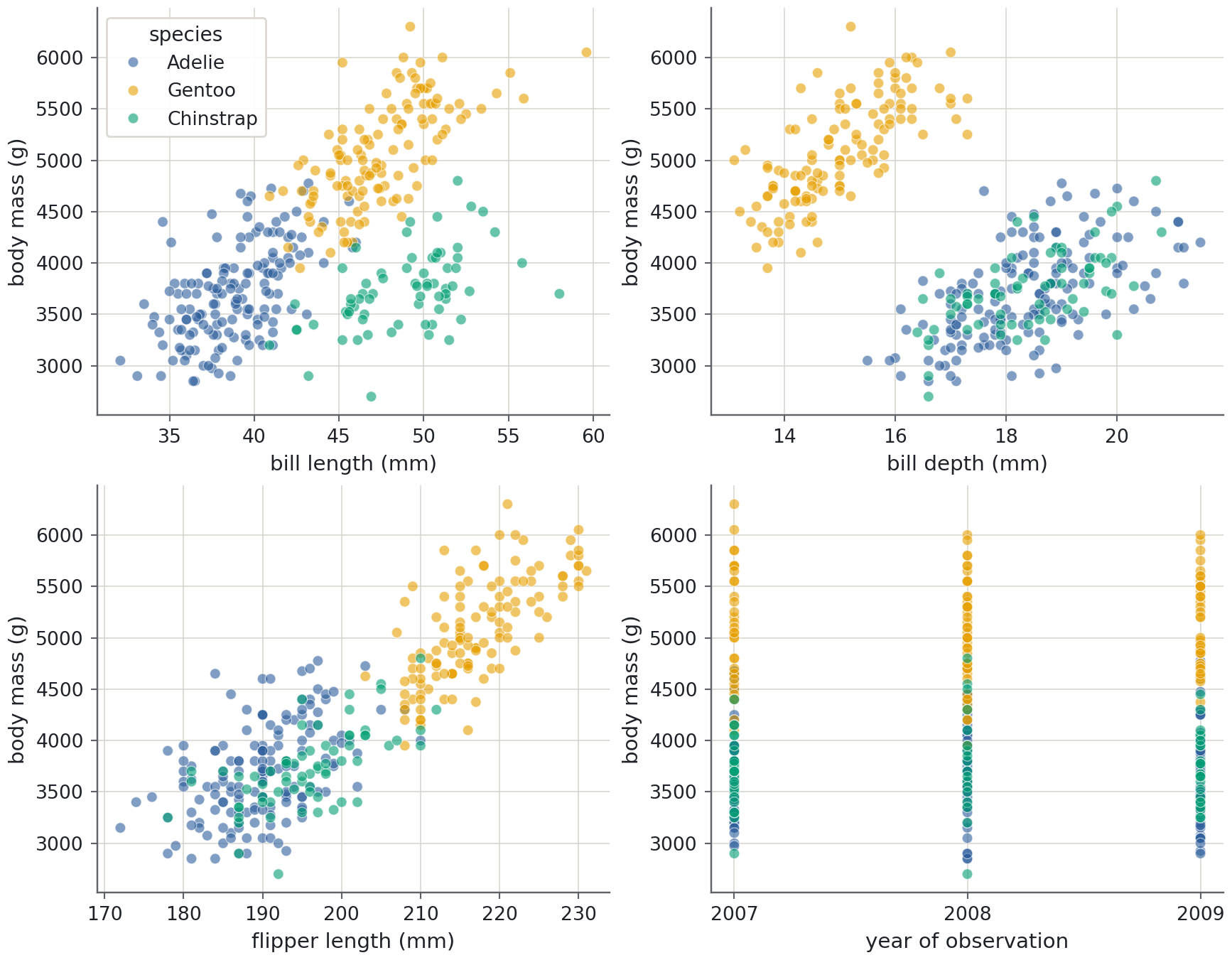
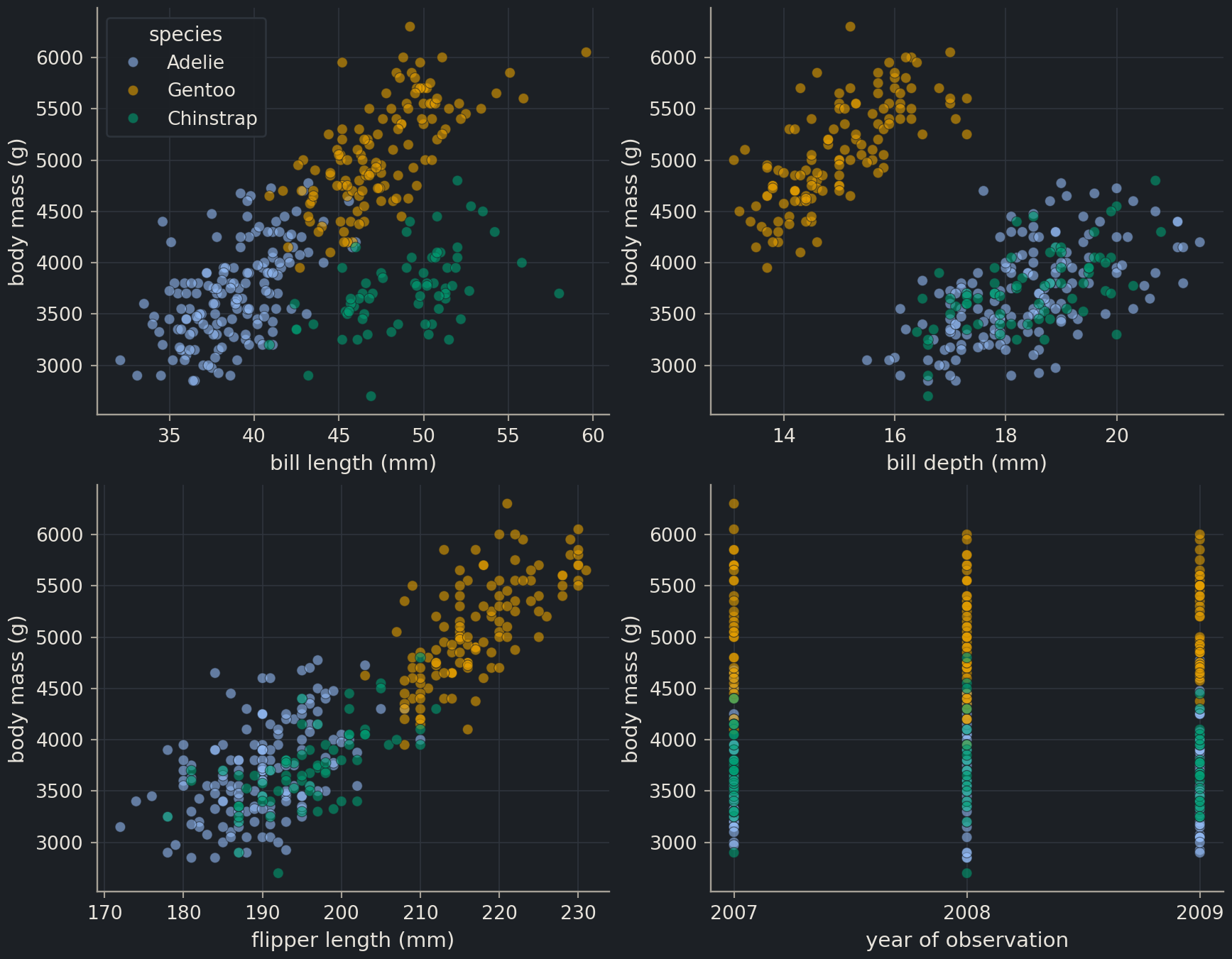
Draw a 2 × 2 grid of scatter plots of body mass against each of the four measurements (bill length, bill depth, flipper length, and body mass against itself is dull, so use year as the fourth x variable instead), coloured by species. Use plt.subplots(2, 2, figsize=(9, 7)) and loop over axes.flat together with the column names. Give every panel labelled axes with units, and show one legend only.
axes.flat iterates over the 2 × 2 array in reading order, zip pairs each panel with a column, and enumerate counts the panels so that legend=(i == 0) draws the legend on the first panel only. The same colours mean the same species in every panel, so repeating the legend four times would add clutter without information. The year panel is deliberately dull: three vertical stripes with no trend. Checking that a bookkeeping column carries no signal is a legitimate use of a plot.
Exercise★★☆
Pairplot for one species
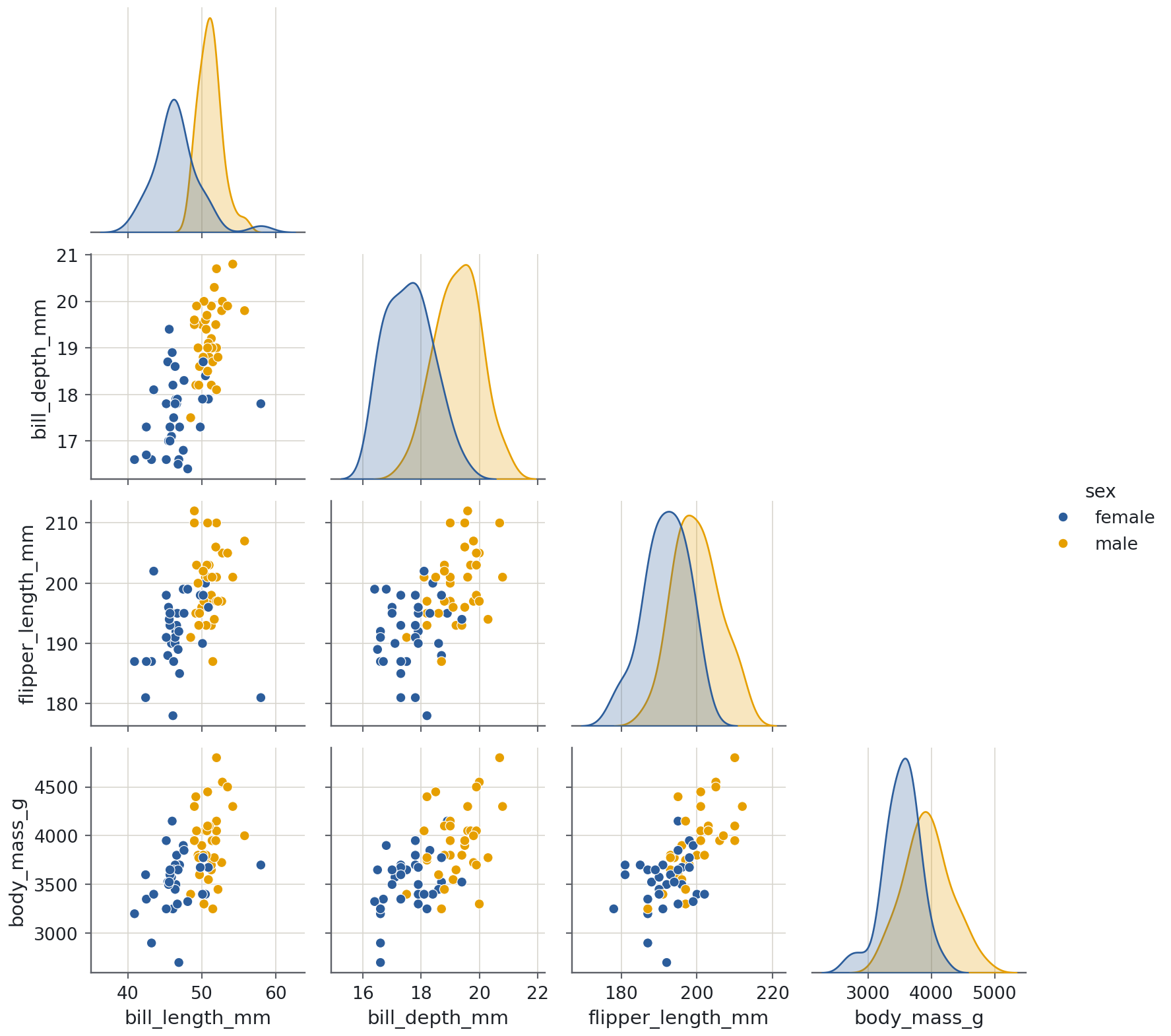
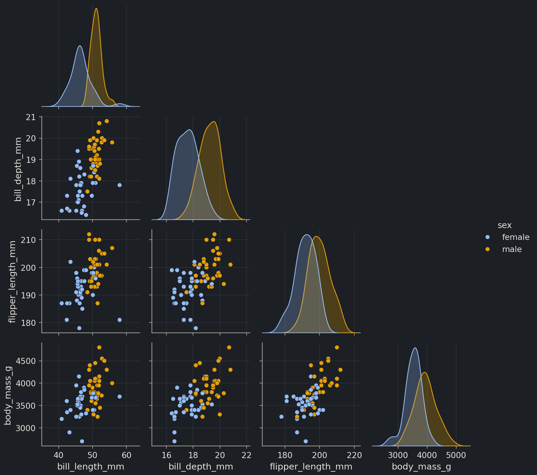
Chinstrap penguins were the hardest to separate from Adelie. Restrict the data to Chinstrap and draw a pairplot of the four measurements coloured by sex. Do male and female Chinstrap penguins separate on any pair of measurements?
Yes, mostly. Males are larger on every measurement, but no single one is clean: bill depths between about 17.5 and 19.5 mm occur in both sexes. The panel of bill depth against bill length does much better, because males are both deeper- and longer-billed, and only a handful of birds sit on the wrong side of the divide. Within a single species the measurements are also positively correlated with each other, which is the “within-group” relationship that the all-species heatmap averaged away. Filtering with a boolean mask (episode 1.3) before plotting is a habit worth keeping: most questions about a dataset are questions about a subset of it.
Exercise★★★
Annotate the heaviest penguin
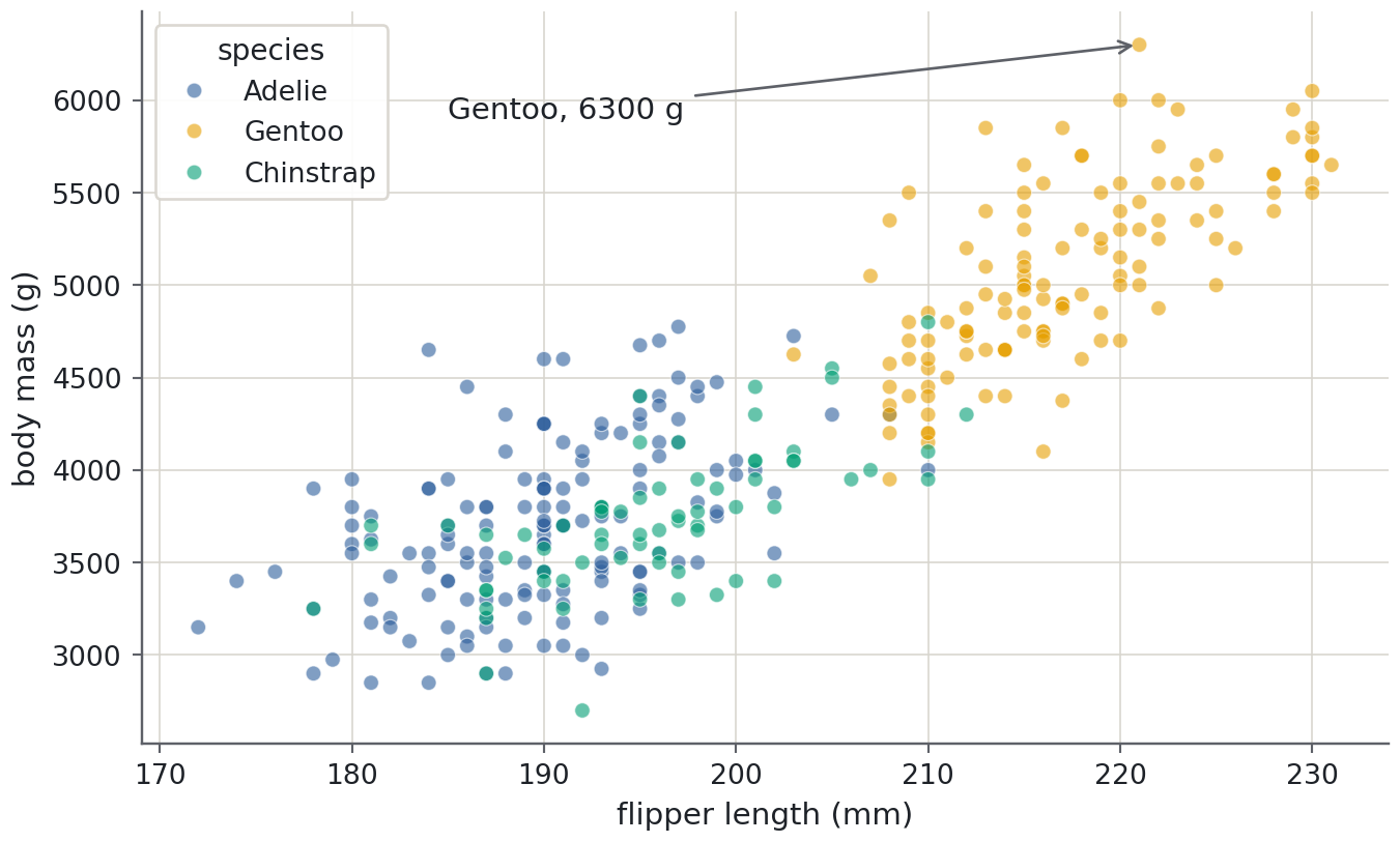
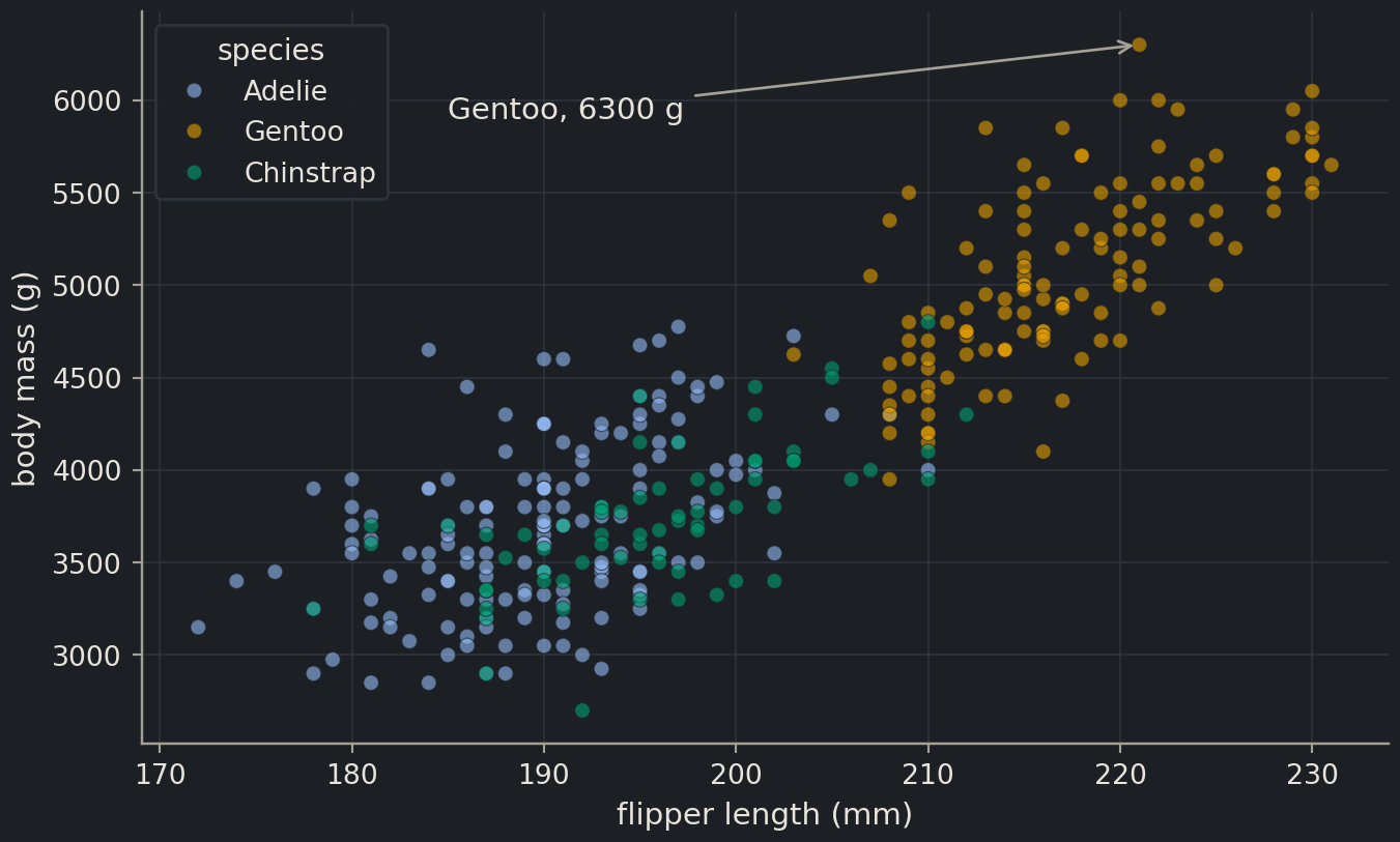
Redraw the scatter plot of body mass against flipper length coloured by species, then find the heaviest penguin with idxmax() and mark it with ax.annotate, giving the species and mass in the label and an arrow pointing at the marker. Look up ax.annotate in the matplotlib documentation; you need the xy, xytext and arrowprops arguments.
idxmax() returns the index label of the largest value, and .loc fetches that row as a Series, so heaviest["species"] and the measurements are one lookup away. xy is the point the arrow touches, in data coordinates; xytext is where the text sits, chosen by hand to land in empty space. Annotating the one point that matters is far more effective than a paragraph describing it, and it is how you flag an outlier to a collaborator without accusing the data of anything yet.
Where this is going
The next episode, 1.5, turns these plots on a chemical dataset: the histogram becomes the distribution of measured solubility, the scatter plots become solubility against molecular weight and polar surface area, and the heatmap tells you which descriptors are worth feeding to a model. From Chapter 2 on, two further figures join the set, the parity plot and the residual plot of episode 2.3, both built with the same fig, ax = plt.subplots() pattern. In Part II the points become molecules and the clusters become chemical series, and the overplotting pitfall becomes a daily concern.
Key points
Plot first, summarise second: a histogram or scatter plot shows shape, outliers and gaps that a mean and a standard deviation hide.
Always create figures with fig, ax = plt.subplots() and draw on ax. The stateful plt.plot interface is for one-off sketches, not for work you will reuse.
One variable: histogram (with a KDE if the sample is large enough). One variable per group: box plot or violin. Two variables: scatter. Many variables: pairplot and a correlation heatmap.
seaborn’s axes-level functions take ax=; figure-level functions such as pairplot build their own figure, so call them alone in a cell.
Label every axis with its unit, give every figure a title or caption, and use a colour-blind-safe palette. Never encode a contrast as red against green.
fig.savefig(“name.png”, dpi=150) writes exactly the figure you see; bbox_inches=“tight” stops labels being cut off.