2.4 Overfitting, regularisation and cross-validation
45 min of teaching25 min of exercisesbeginner
Questions this episode answers
Why does a more flexible model often predict worse on new data?
How do I tell whether my model is too simple or too flexible, and what do I do about it?
What does regularisation actually change in a linear model?
How do I choose a setting like the regularisation strength without cheating with the test set?
What you will be able to do
Recognise underfitting and overfitting from training and test errors, and from learning and validation curves.
Explain the bias–variance trade-off in words and connect it to model flexibility.
Fit ridge and lasso models in a scaled pipeline and read how the penalty shrinks or removes coefficients.
Estimate a model’s error with k-fold cross-validation and report it as mean ± standard deviation.
Tune a hyperparameter with GridSearchCV and evaluate the chosen model on the test set exactly once.
The residual plot at the end of episode 2.3 exposed large errors for some molecules. A more flexible model is one possible response. The trap is that flexibility has no natural stopping point. A model that can bend to the signal can also bend to the noise, and from the training error alone you cannot tell which it is doing. This episode gives you the tools to tell the difference, a dial (regularisationregularisationAdding a penalty on large coefficients so that a model stays simpler and generalises better.) that sets the flexibility deliberately, and a procedure (cross-validationcross-validationRepeatedly splitting the data into folds so that every sample is tested on exactly once.) for setting that dial without touching the test set.
A controlled experiment: curves of increasing flexibility
Real descriptors are messy, so start with data where you know the truth. The cell below draws 30 points from a smooth curve, \(\sin(2\pi x)\), adds Gaussian noise, and splits them as in episode 2.3.
A straight line cannot follow a sine wave. One way to let a linear model bend is to hand it polynomial featurespolynomial featuresNew features made from powers and products of the originals, letting a linear model fit curves.: alongside \(x\) it also receives \(x^2, x^3, \dots, x^d\) and fits one coefficient per power. The degree \(d\) controls how much the curve can wiggle. We first centre and scale \(x\) to keep the high powers numerically stable, then use PolynomialFeatures(d, include_bias=False) to build the powers; LinearRegression supplies the intercept. make_pipeline chains these steps into one object that fits and predicts (pipelines get their own treatment in episode 2.6).
Predict before you run
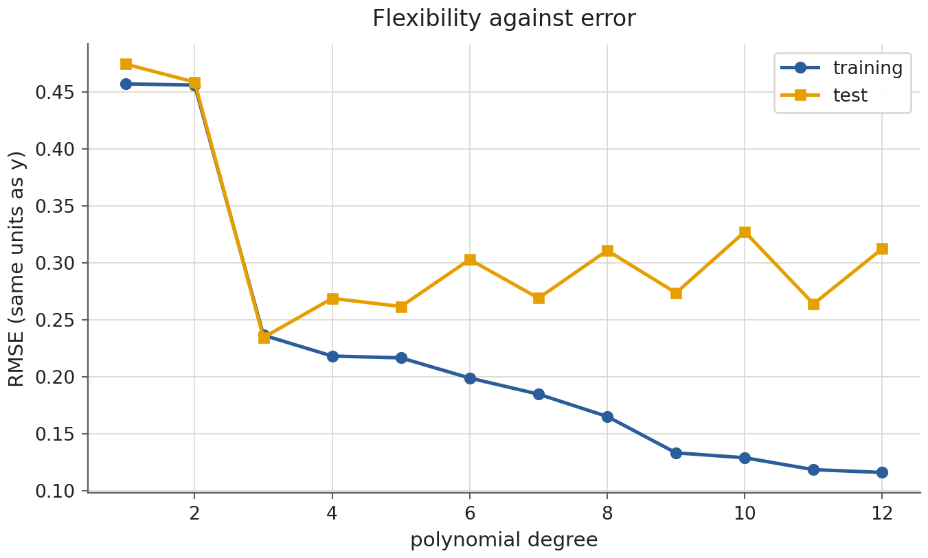
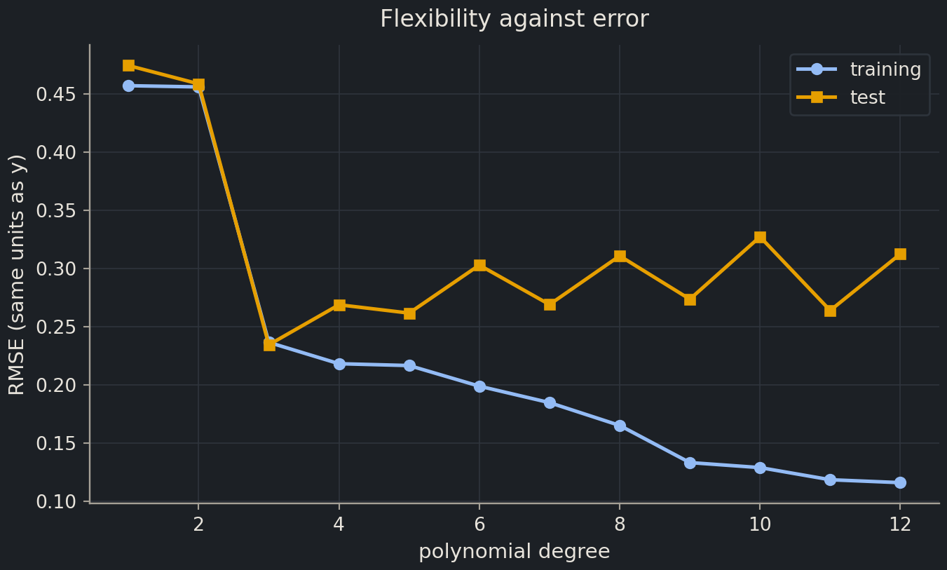
Before you run the next cell: as the degree goes from 1 to 12, what happens to the training RMSE? And to the test RMSE? Sketch both curves.
import matplotlib.pyplot as pltfig, ax = plt.subplots()ax.plot(curve.index, curve["train RMSE"], marker="o", label="training")ax.plot(curve.index, curve["test RMSE"], marker="s", label="test")ax.set(xlabel="polynomial degree", ylabel="RMSE (same units as y)", title="Flexibility against error")ax.legend()plt.show()
The two curves tell the whole story of this episode:
Training error only goes down here. A degree-12 polynomial has 13 coefficients and 21 training points. Each higher-degree model can reproduce any lower-degree fit by setting its extra coefficient to zero, so the best least-squares training fit cannot get worse.
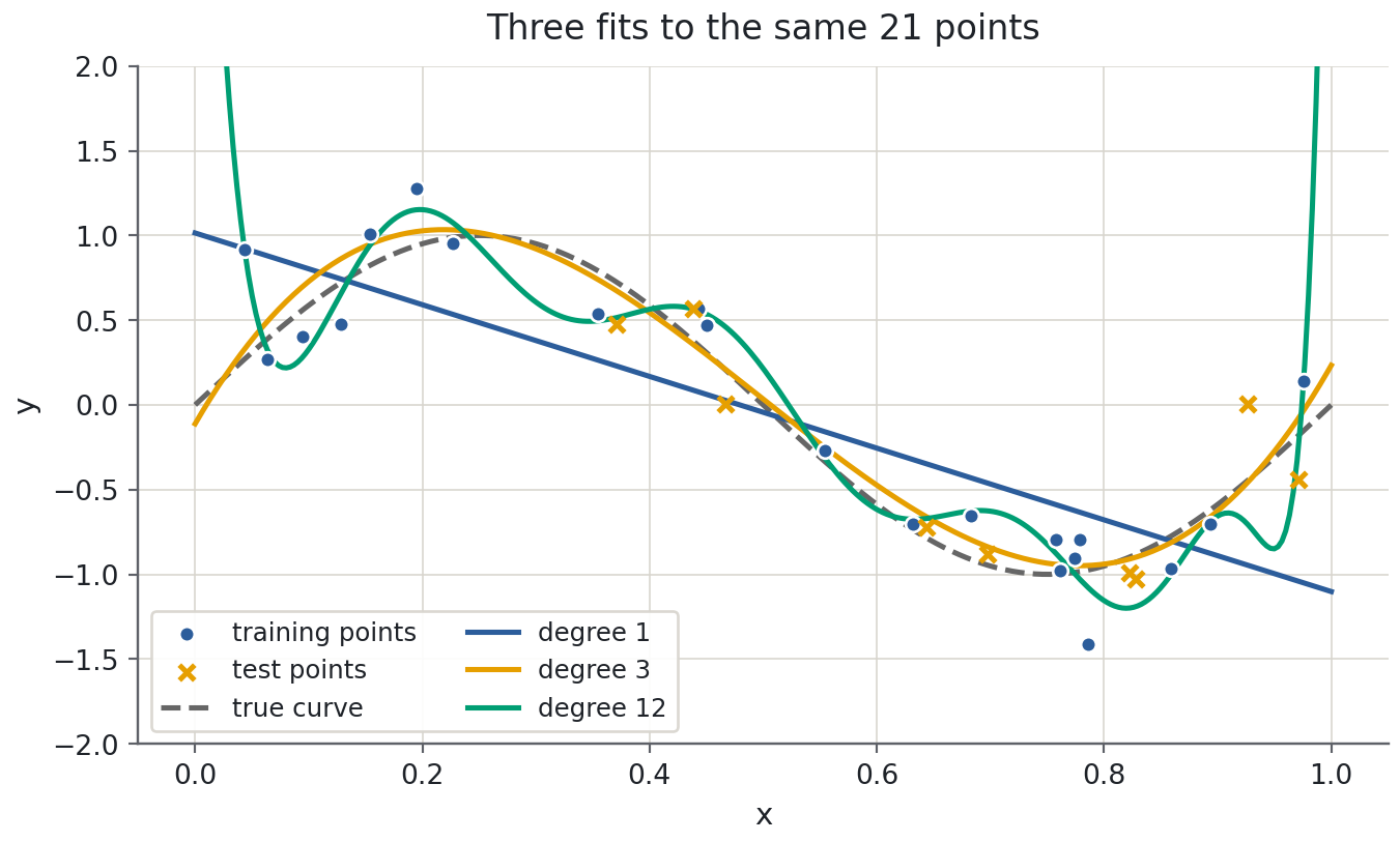
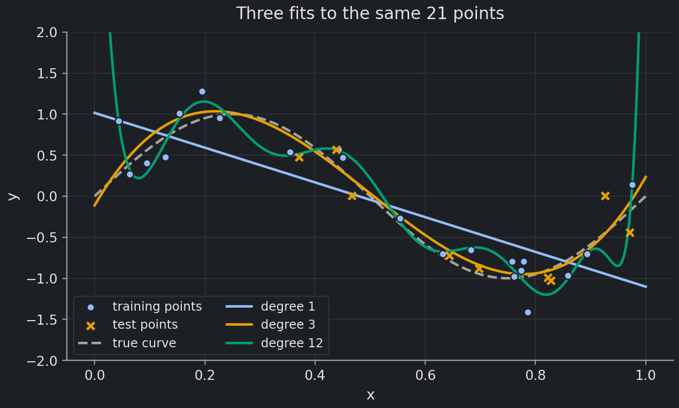
Test error has a minimum. Degrees 1 and 2 are too rigid: that is underfittingunderfittingWhen a model is too simple to capture the real pattern, so it does badly even on training data., and both errors are high. Degree 3 has the lowest test error in this split. Higher degrees have larger test errors, with some fluctuations, while training error keeps falling: that is overfittingoverfittingWhen a model learns the noise in its training data and so performs worse on new data.. With only nine test points, the curve is not a smooth textbook U.
Look at three of the fits to see what the numbers mean.
Degree 12 is the student from episode 2.3 who memorised last year’s exam. It passes close to every training point, noise included, and between the points it swings to values the true curve never takes. The test points, which it has not seen, land far from its swings.
Common mistake
Flexibility is not the number of inputs
The degree-12 model has one input but 13 coefficients. A QSAR model with five descriptors and interaction terms, or a neural network, is likewise far more flexible than its input count suggests. Judge flexibility by the number of free parametersparameterA number inside a model that training adjusts, such as a regression coefficient. relative to the number of training samples that constrain them.
Bias and variance
The U shape has a name: the bias–variance trade-offbias–variance trade-offSimple models err by being too rigid (bias); flexible models err by following noise (variance).. Imagine repeating the experiment many times, each with a fresh noisy sample of 30 points, and fitting the same kind of model to each.
A rigid model (degree 1) gives nearly the same line every time. Its predictions are stable but systematically wrong, because a line cannot be a sine wave. That systematic error is bias.
A flexible model (degree 12) gives a different curve every time, because it follows whichever noise it happened to see. Averaged over repetitions it might be about right; any single fit is far from the truth. That instability is variance.
Increasing flexibility lowers bias and raises variance. The test error is the sum of both, plus the noise no model can remove, which is why it has a minimum in the middle. Everything that follows is a way of finding that minimum on purpose rather than by luck.
Deep diveThe bias–variance decompositionShow the mathsHide the maths
Suppose \(y = f(x) + \varepsilon\) with \(\mathbb{E}[\varepsilon] = 0\) and \(\operatorname{Var}(\varepsilon) = \sigma^2\), and let \(\hat{f}\) be the model fitted to a random training set. For a fixed input \(x\), the expected squared error over training sets and noise is
The proof adds and subtracts \(\mathbb{E}[\hat{f}(x)]\) inside the square; the cross terms vanish because \(\varepsilon\) is independent of the training set. The decomposition is exact for squared error and holds qualitatively for other losses.
Chemist's corner
A QSAR model with 200 descriptors fitted to 50 compounds will overfit, however carefully the descriptors were chosen: with more coefficients than measurements, a linear model reproduces the training activities exactly, noise included, and its prediction for the next compound is close to random. Regularisation is the standard answer, and this episode is the toolkit QSAR practitioners use. A random split flatters such a model, because test compounds are near-copies of training compounds; a scaffold splitscaffold splitSplitting molecules so that chemically similar scaffolds do not appear in both train and test. (Chapter 6) moves the whole test curve up and makes it honest.
Biologist's corner
Gene-expression studies are the extreme case: 20,000 genes measured in 100 samples, so the number of features \(p\) vastly exceeds the number of samples \(n\). Any unregularised linear model fits such data perfectly and means nothing. The lasso below is popular there because it returns a short list of genes with non-zero coefficients, which a biologist can follow up.
Two diagnostic curves on real data
Back to the solubility data and the five descriptors from episode 2.3, with the same split so the numbers are comparable.
from pathlib import PathESOL_URL ="https://deepchemdata.s3-us-west-1.amazonaws.com/datasets/delaney-processed.csv"path = Path("data/esol.csv")esol = pd.read_csv(path if path.exists() else ESOL_URL)features = ["Molecular Weight","Number of H-Bond Donors","Number of Rings","Number of Rotatable Bonds","Polar Surface Area",]X = esol[features]y = esol["measured log solubility in mols per litre"]X_train, X_test, y_train, y_test = train_test_split(X, y, test_size=0.2, random_state=42)
The learning curve: would more data help?
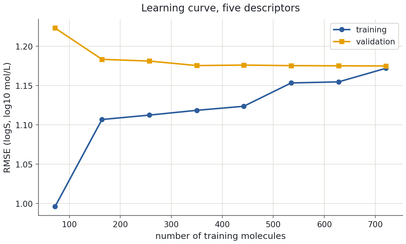
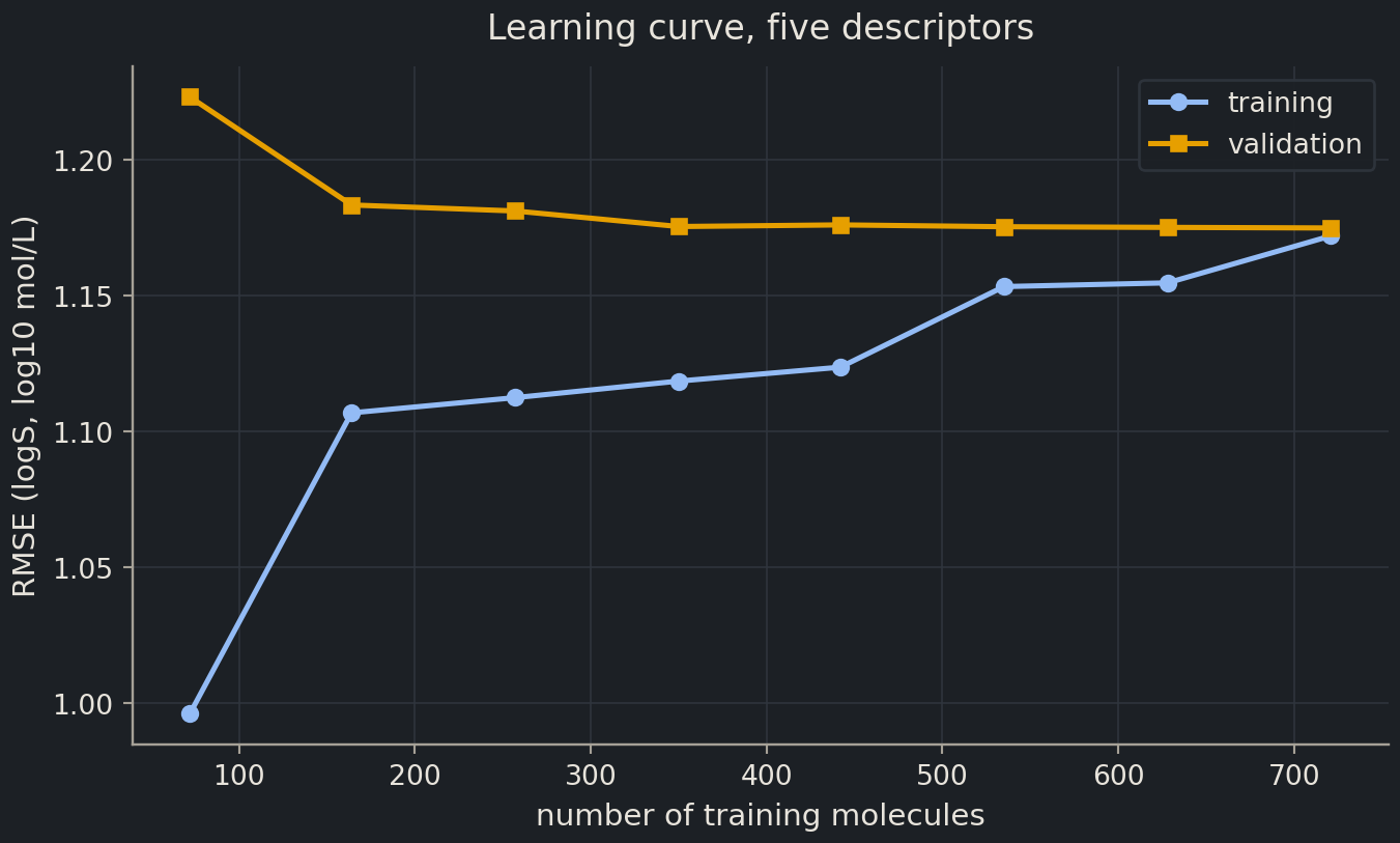
A learning curvelearning curveTraining and validation scores plotted against the amount of training data. fits the model on growing fractions of the training set and records, for each size, the error on the data it trained on and on data it did not. learning_curve does the bookkeeping. cv=5 means each size is tried five times on different subsets (that is cross-validation, explained properly below) and averaged. Scoring is "neg_root_mean_squared_error": scikit-learn’s convention is that higher is better for every score, so errors come back with a minus sign, and we negate them back. The model is a Ridge inside a scaled pipeline; for now read it as “linear regression”, and the reason for the two extra pieces is coming.
fig, ax = plt.subplots()ax.plot(sizes, train_rmse, marker="o", label="training")ax.plot(sizes, val_rmse, marker="s", label="validation")ax.set(xlabel="number of training molecules", ylabel="RMSE (logS, log10 mol/L)", title="Learning curve, five descriptors")ax.legend()plt.show()
Read a learning curve by asking two questions. Have the curves converged? Yes: beyond about 250 molecules the validation error stops improving and the training error has risen to meet it. More ESOL molecules would not help this model. Where have they converged? At about 1.18 log units, well above the measurement noise. Training and validation errors that are both high and equal mean underfitting: the limit is bias, not data. The cure is a better representation of the molecule (Part II) or a more flexible model (Chapter 3), not more rows. Had the curves still been far apart at the right-hand edge, the diagnosis would be overfitting, and more data would be the first thing to try.
The validation curve: how should a setting be chosen?
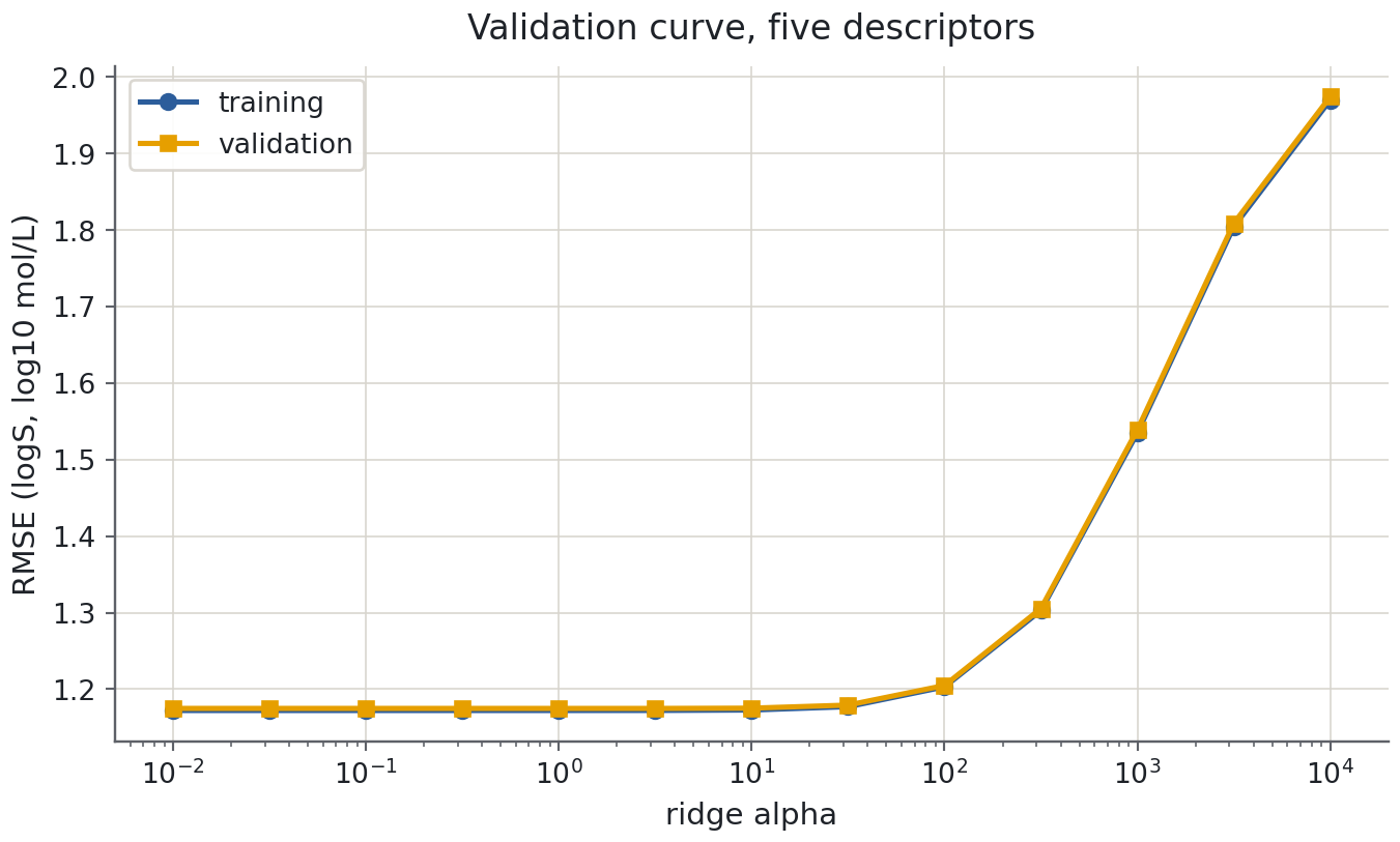
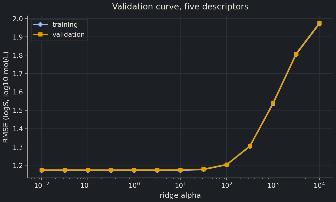
Ridge has an argument alpha that we did not learn from the data. It is a hyperparameterhyperparameterA setting chosen before training, such as the number of neighbours in kNN or the strength of regularisation., a setting fixed before fitting, unlike the coefficients, which are parameters that fitting adjusts. A validation curvevalidation curveTraining and validation scores plotted against one hyperparameter. plots training and validation error against one hyperparameter. The name "ridge__alpha" is how scikit-learn reaches into a pipeline: step name, two underscores, argument.
Flat, then rising: small alpha changes nothing, large alpha hurts. Five descriptors fitted to 900 molecules have nothing to overfit, so there is nothing for the penalty to fix. Keep this picture in mind; shortly you will see the same curve for a model that does overfit, and it will have the U from the synthetic experiment.
Regularisation: ridge and lasso
What does alpha do? Ordinary least squares finds the coefficientscoefficientThe weight a linear model gives to one feature; its sign and size are only interpretable with care.\(w\) that minimise the squared error. Ridge regressionridge regressionLinear regression with an L2 penalty that shrinks coefficients towards zero. minimises the squared error plus a penalty\(\alpha \sum_j w_j^2\) on the size of the coefficients. The penalty pulls every coefficient towards zero; alpha sets how hard. Large coefficients are what let a model swing between data points, so shrinking them reduces variance at the cost of a little bias. Lassolasso regressionLinear regression with an L1 penalty that sets some coefficients exactly to zero (feature selection). does the same with the penalty \(\alpha \sum_j |w_j|\), and that small change has a large consequence.
Why the scaler comes first
A penalty on coefficient size only makes sense if the coefficients are comparable. Molecular weight runs from about 16 to 780 g/mol; the number of H-bond donors from 0 to about 11. A coefficient on weight is “logS per g/mol” and naturally tiny; one on donors is “logS per donor” and naturally larger. Penalising both by the same rule would punish the donor coefficient for its units, not its importance. feature scalingfeature scalingTransforming features to comparable ranges, such as zero mean and unit variance. fixes this: StandardScaler rescales each feature to mean 0 and standard deviation 1, so every coefficient is “logS per standard deviation of the feature” and the penalty treats them fairly. Episode 2.6 explains why the scaler must live inside the pipeline; for now, never fit a penalised model on raw descriptors.
Ridge shrinks
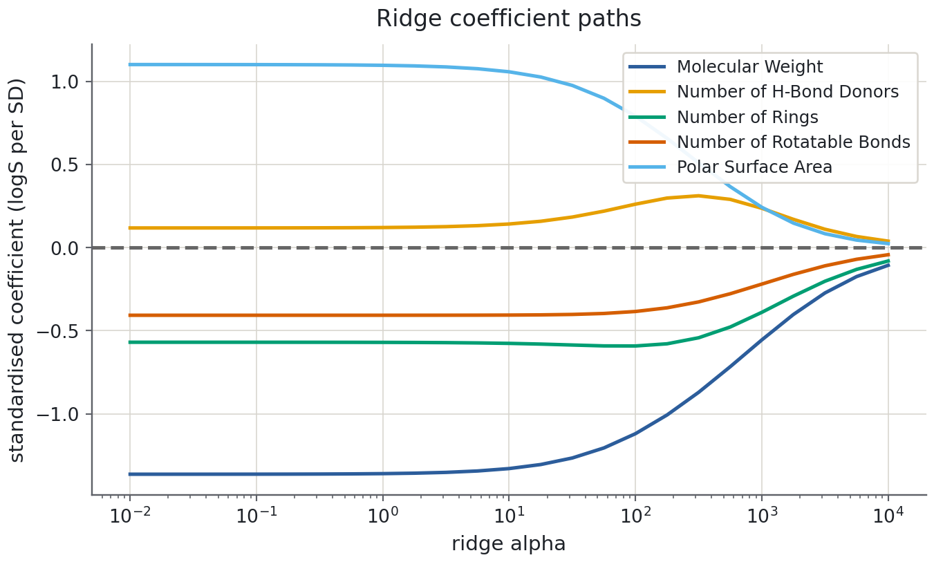
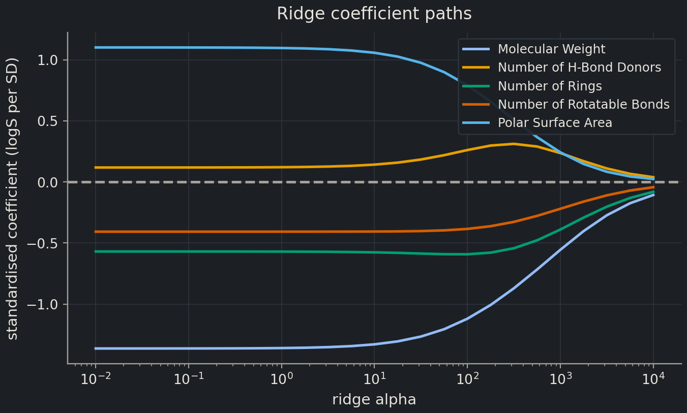
Fit ridge for a range of alpha values and collect the five coefficients each time. ridge[-1] is the last step of the pipeline, the Ridge object, whose coef_ holds the fitted coefficients.
alphas = np.logspace(-2, 4, 25)coef_paths = pd.DataFrame( [make_pipeline(StandardScaler(), Ridge(alpha=a)).fit(X_train, y_train)[-1].coef_ for a in alphas], index=alphas, columns=features,)coef_paths.iloc[::6].round(3)
index
Molecular Weight
Number of H-Bond Donors
Number of Rings
Number of Rotatable Bonds
Polar Surface Area
0.010000
-1.363
0.118
-0.569
-0.407
1.100
0.316228
-1.362
0.119
-0.570
-0.407
1.099
10.000000
-1.329
0.142
-0.576
-0.406
1.057
316.227766
-0.870
0.311
-0.543
-0.327
0.509
10000.000000
-0.107
0.039
-0.081
-0.043
0.024
fig, ax = plt.subplots()for name in features: ax.plot(coef_paths.index, coef_paths[name], label=name)ax.axhline(0, color="0.4", linestyle="--")ax.set(xscale="log", xlabel="ridge alpha", ylabel="standardised coefficient (logS per SD)", title="Ridge coefficient paths")ax.legend(fontsize="small")plt.show()
At small alpha the coefficients are close to ordinary least squares: heavier molecules and more rings are associated with lower solubility, and more polar surface area with higher solubility. Increasing alpha shrinks the overall coefficient norm, but individual coefficients need not shrink at every step when descriptors are correlated: the H-bond donor coefficient first grows. All five approach zero at large alpha; ridge does not deliberately select coefficients to set exactly to zero.
Maths corner
Ridge has two equivalent readings. As a constrained problem it is least squares subject to \(\|w\|_2^2 \le t\): the solution is the point of a ball closest to the unconstrained optimum, hence shrinkage. As a Bayesian estimate it is the posterior mode (MAP) under a Gaussian prior \(w_j \sim \mathcal{N}(0, \tau^2)\) with \(\alpha = \sigma^2 / \tau^2\): the prior says “coefficients are probably small” and alpha is how strongly you believe it. The closed form is \(\hat{w} = (X^\top X + \alpha I)^{-1} X^\top y\); the \(\alpha I\) term is what makes the inverse exist when \(p > n\).
Lasso selects
Predict before you run
Lasso’s penalty is \(\alpha \sum_j |w_j|\) rather than \(\alpha \sum_j w_j^2\). Before you run the next cell, guess which descriptor’s coefficient disappears first as alpha grows, and whether the others shrink smoothly or stay put.
from sklearn.linear_model import Lassolasso_alphas = [0.001, 0.05, 0.1, 0.2, 0.5, 1.0]lasso_paths = pd.DataFrame( [make_pipeline(StandardScaler(), Lasso(alpha=a)).fit(X_train, y_train)[-1].coef_ for a in lasso_alphas], index=pd.Index(lasso_alphas, name="alpha"), columns=features,)lasso_paths.round(3)
index
Molecular Weight
Number of H-Bond Donors
Number of Rings
Number of Rotatable Bonds
Polar Surface Area
alpha
index
index
index
index
index
0.001
-1.363
0.118
-0.568
-0.405
1.098
0.050
-1.362
0.124
-0.471
-0.313
0.986
0.100
-1.360
0.129
-0.372
-0.218
0.871
0.200
-1.357
0.141
-0.175
-0.029
0.642
0.500
-0.909
0.092
-0.000
-0.000
0.096
1.000
-0.340
0.000
-0.000
0.000
0.000
Read down the rows. By alpha = 0.5 the coefficients of Number of Rings and Number of Rotatable Bonds are exactly zero: lasso has dropped those descriptors from the model. By alpha = 1.0 only molecular weight survives. This is the sparsity effect: lasso performs feature selection as a side effect of fitting, and the order in which descriptors vanish ranks how much independent information each carries about solubility. Ridge never does this; its coefficients approach zero but every feature stays in play.
Deep diveWhy L1 gives exact zeros and L2 does notShow the mathsHide the maths
Write both penalties as constraints: minimise the squared error subject to \(\sum_j |w_j| \le t\) (lasso) or \(\sum_j w_j^2 \le t\) (ridge). In two dimensions the lasso region is a diamond with corners on the axes; the ridge region is a disc. The squared error forms elliptical contours around the unconstrained optimum, and the solution is where the smallest contour touches the region. An ellipse touches a disc at a point with both coordinates non-zero almost surely; it very often touches a diamond at a corner, where one coordinate is exactly zero. In \(p\) dimensions the diamond has corners, edges and faces on every coordinate subspace, so whole groups of coefficients vanish. Equivalently: the subgradient of \(|w_j|\) at zero is the interval \([-\alpha, \alpha]\), which can absorb a small error gradient and hold the coefficient at zero; the derivative of \(w_j^2\) at zero is zero and cannot.
When regularisation matters: small data
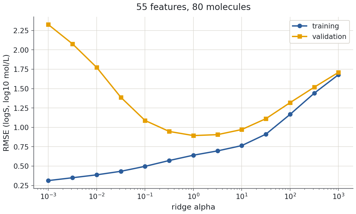
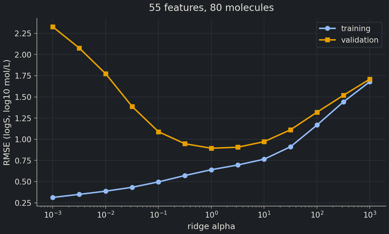
The validation curve above was flat because 900 molecules and five descriptors cannot overfit. Make the problem hard in the way real projects are hard: expand the five descriptors into all products up to degree 3 (55 features) and keep only the first 80 training molecules, a typical size for a medicinal-chemistry series. The scaler now sits after the expansion, so that the squared and cubed features are standardised too.
Now the U is back. With almost as many features as molecules, the barely regularised fit has a training RMSE of 0.3 and a validation RMSE of 2.3: it has memorised 80 molecules and knows little about the 81st. A penalty of alpha around 1 cuts the validation error to about 0.9; too much penalty and the model slides into underfitting on the right. The validation curve is how you find the sweet spot, and the rest of the episode is how to do that systematically. (Whether 0.9 is believable for molecules unlike these 80 is the stretch exercise, and the answer is sobering.)
For programmers
Parameters are what fit writes (coef_, intercept_); hyperparameters are constructor arguments (alpha, degree, n_neighbors) that fit reads but never changes. Tuning is therefore an outer loop around fit: for alpha in grid: for fold in folds: fit, score. GridSearchCV below is exactly that nested loop plus bookkeeping, with n_jobs=-1 to run iterations in parallel. Treat the grid as part of your experiment’s configuration and log it with the results.
Cross-validation: k splits instead of one
Episode 2.3 ended with ten random splits giving ten different RMSEs. A single split is one noisy draw from that distribution. k-fold cross-validation makes the draws systematic: shuffle the training data once, cut it into \(k\) equal folds, and for each fold in turn fit on the other \(k-1\) and score on the held-out one. Every sample is scored exactly once by a model that never saw it, and you get \(k\) scores whose mean and spread you can report.
Three details matter. KFold carries shuffle=True and random_state=42: without shuffling the folds are consecutive blocks of rows, a disaster if the file is sorted by anything. The scores come back negative because of the higher-is-better convention; flip the sign before reporting. And the standard deviation of about 0.1 is the honest uncertainty on the 1.19: two models whose cross-validated RMSEs differ by 0.02 are not distinguishable on this data.
Common mistake
Cross-validation does not replace the test set
Cross-validation here runs on X_train only. Its job is to make decisions (which model, which alpha) without the test set, whose whole value is that no decision was ever made with it. If you cross-validate on the full dataset and then report “test” numbers from the same rows, the test numbers are contaminated.
Choosing hyperparameters with grid search
A grid searchgrid searchTrying every combination of candidate hyperparameter values and keeping the best by cross-validation. tries every candidate value of a hyperparameter, cross-validates each, and keeps the one with the best mean score. GridSearchCV wraps a model and a dictionary of candidates; after fit it behaves like the best model, refitted on all of the training data.
best alpha: {'ridge__alpha': np.float64(10.0)}
best cross-validated RMSE: 1.188
Look at the full table in cv_results_ before trusting best_params_: a winner that beats its neighbours by less than the fold-to-fold spread is a coin toss.
As the validation curve predicted, every alpha up to about 30 scores the same within the spread, and the “best” wins by a thousandth. That is a legitimate conclusion: regularisation does not matter for this model, and any small alpha is fine. The same search for lasso returns the same verdict and keeps all five descriptors.
best alpha: {'lasso__alpha': np.float64(0.0001)}    best CV RMSE: 1.189
non-zero coefficients: 5 of 5
Now, and only now, the test set. grid.predict uses the refitted best model. This is the number you would put in a report, computed once.
test_rmse = root_mean_squared_error(y_test, grid.predict(X_test))print(f"test RMSE of the chosen ridge model: {test_rmse:.3f}")
test RMSE of the chosen ridge model: 1.214
It agrees with the cross-validated estimate within the spread, which is the reassurance you want: the selection procedure did not fool itself. It is also, within noise, the plain linear model’s 1.21 from episode 2.3, as it should be.
Common mistake
best_score_ is not the test score
best_score_ is the cross-validated score of the winning candidate. Because it is the maximum over the grid it is slightly optimistic, in the way the best of ten lottery tickets looks luckier than a typical one. Report it as “cross-validated” and report the untouched test set separately. The Debug exercise shows how this mistake usually looks.
Train, validation, test
The data flow of a complete project, as a picture in words:
Split once into training and test. Put the test set in a drawer.
Inside the training set, use cross-validation to compare models and tune hyperparameters. Each fold’s held-out part plays the role of a validation setvalidation setData held back from training that you use to choose between models or settings.: data the model did not fit on, used to make a decision.
Refit the chosen model on all of the training data.
Open the drawer and score the refitted model on the test set once. If the number disappoints you, you do not get to return to step 2 with the test set in view; that would turn it into another validation set.
On large datasets people often replace the cross-validation in step 2 with one fixed validation split (train / validation / test, often 60 / 20 / 20), which is cheaper and fine when every part has thousands of rows. On the small datasets common in chemistry and biology, cross-validation is worth its cost.
Note
Nested cross-validation
Step 4 checks the whole procedure, grid search included. When the data are too small to spare a test set, nested cross-validationnested cross-validationCross-validation inside cross-validation, so that hyperparameter tuning does not bias the final estimate. does the same job: an outer cross-validation loop scores the procedure, and inside each outer fold an inner GridSearchCV chooses the hyperparameters. In scikit-learn that is one line, cross_val_score(GridSearchCV(...), X, y, cv=outer). It matters when \(n\) is tens, not thousands.
Exercises
Exercise★☆☆
Underfitting or overfitting?
For each situation, say whether the model is underfitting, overfitting, or neither, and name one change that would help.
Training RMSE 0.20, test RMSE 1.40.
Training RMSE 1.20, test RMSE 1.25, and the learning curve has flattened.
Training RMSE 0.90, test RMSE 0.95, and the validation error is still falling as training data are added.
Cross-validated RMSE 1.19 ± 0.10 for alpha = 1 and 1.18 ± 0.10 for alpha = 10.
SolutionShow solutionHide solution
Overfitting: a large train–test gap. Increase regularisation, reduce the number of features, or get more data.
Underfitting: both errors high and equal, and more data would not help. Use a more flexible model or better features.
Neither, but data-limited: the gap is small and the validation error still improves with data, so collect more samples before changing the model.
Not distinguishable: the difference of 0.01 is a tenth of the fold-to-fold spread. Either alpha is fine; say so rather than claiming alpha = 10 is “better”.
Exercise★☆☆
Debug this
A colleague’s report says “our ridge model achieves a test RMSE of 1.05”. Their code runs without errors. Find the two problems.
The scaler sees the test set.StandardScaler().fit(X) computes means and standard deviations from all rows, including those that become the test set, a mild form of data leakagedata leakageWhen information from outside the training set sneaks into the model, making evaluation misleadingly good.. Put the scaler inside the pipeline, make_pipeline(StandardScaler(), Ridge()), and split the raw data; the pipeline then fits the scaler on the training part only, inside every cross-validation fold too.
best_score_ is reported as the test score. It is the cross-validated score of the best candidate, measured on training data and optimistically selected as the maximum over the grid. The test set was never used. Report root_mean_squared_error(y_test, grid.predict(X_test)) as the test RMSE and -grid.best_score_ separately as the cross-validated RMSE.
Expand the five descriptors to degree 2 with PolynomialFeatures(2, include_bias=False) (20 features: the originals, their squares and pairwise products), scale, and fit a Lasso with alpha=0.05 on the full training set. How many coefficients are non-zero, and which features survive? (pipeline[:-1].get_feature_names_out() gives the expanded names.) Compare the test RMSE with the five-descriptor ridge model.
10 of 20 coefficients are non-zero
Molecular Weight                                    -1.412
Polar Surface Area                                   0.839
Number of Rings                                     -0.638
Number of Rings Polar Surface Area                   0.371
Number of Rotatable Bonds                           -0.258
Number of Rotatable Bonds^2                         -0.112
Number of H-Bond Donors Number of Rotatable Bonds    0.075
Polar Surface Area^2                                -0.057
Number of Rings Number of Rotatable Bonds            0.052
Number of H-Bond Donors                              0.039
dtype: float64
test RMSE: 1.190
Half of the twenty features are dropped. The survivors are led by the original descriptors (weight, polar surface area, rings) with a few products and squares behind them, and the test RMSE edges below the five-descriptor model’s 1.21: the extra terms let the model bend, the penalty stops it from using all twenty to chase noise, and lasso reports afterwards which of the added terms were worth having.
Exercise★★★
Nested CV, and what cross-validation cannot see
Using small_X, small_y (80 molecules) and the poly_ridge pipeline, run GridSearchCV over ridge__alpha in np.logspace(-3, 3, 13) with cv=cv and record -best_score_. Then estimate the same procedure with nested cross-validation, cross_val_score(GridSearchCV(...), small_X, small_y, cv=outer) with outer = KFold(5, shuffle=True, random_state=42). Finally score the grid’s refitted best model on the full test set. Compare the three numbers. Which would you put in a paper, and what does the comparison warn you about?
best_score_:   0.918   at {'ridge__alpha': np.float64(3.1622776601683795)}
nested CV:     0.964 ± 0.116
test RMSE:     1.502   (226 molecules)
The nested estimate is a little higher than best_score_, which is the optimism of picking the maximum over 13 candidates, and it is the number to report if you have no test set. But both cross-validated numbers are far below the test RMSE. Cross-validation can only tell you how the model does on molecules like the ones you have: the 80 molecules span a narrower range of weight and polar surface area than the test set, and a cubic polynomial extrapolates violently outside the range it was fitted on, so a handful of test molecules are missed by several log units. Nested CV fixes the optimism of selection; it cannot fix a training set that does not cover the chemistry you will be asked about. That is the applicability-domain problem of Chapter 6.
Where this is going
Every model in the rest of the course has hyperparameters, and every one is chosen the way you did it here: cross-validation inside the training data, the test set opened once. In Chapter 6 the folds and the test set stop being random: a scaffold split puts whole chemical series on one side or the other, so the validation curve answers “how well does this model handle new chemistry?” rather than “how well does it interpolate between near-duplicates?”, and the applicability domain you glimpsed in the stretch exercise becomes something you can measure. In Chapter 7 the grid becomes a search over learning rates, layer widths and dropout for graph neural networks, the same nested loop with a far more expensive fit inside it; the discipline of never letting the test set vote is what keeps those results honest. Episode 2.5 turns to classification, where the bias–variance story reappears as the jagged boundary of a nearest-neighbour model.
Key points
For nested least-squares models, the best training error cannot increase with flexibility; test error can rise as the model starts fitting noise.
Bias is error from being too rigid; variance is error from following noise. Every model choice trades one for the other.
A learning curve says whether more data would help; a validation curve says how a hyperparameter should be set.
Ridge shrinks coefficients smoothly; lasso sets some exactly to zero. Both need scaled features, so put a StandardScaler in the pipeline.
Cross-validation replaces one lucky or unlucky split with k systematic ones; report the mean and the spread.
Choose hyperparameters with cross-validation on the training data; the test set is touched once, at the very end, and never used to choose anything.