How does a model predict a category instead of a number, and where do the probabilities come from?
Why is accuracy a poor summary of a classifier, and what should I report instead?
What changes when the class I care about is rare, as active compounds are in a screen?
What you will be able to do
Train logistic regression and k-nearest-neighbour classifiers in scikit-learn pipelines and read their decision boundaries.
Compute and interpret a confusion matrix, accuracy, precision, recall, F1, ROC/AUC and precision–recall curves.
Choose a decision threshold deliberately rather than accepting 0.5.
Recognise class imbalance and evaluate a classifier on a rare positive class honestly.
So far every model in this chapter has predicted a number. Many scientific questions are not numbers but categories: is this tumour malignant or benign, is this compound active in the assay, is this sequence a signal peptide? That is classificationclassificationPredicting a category, such as active versus inactive., and most of what you learned about regression carries over: features, a model with parameters, a loss, a split, a baseline. What changes is the output, and with it the way you judge the model.
This episode uses the breast cancer Wisconsin dataset that you explored in Lab 1: 569 tumours, 30 features computed from microscope images of a needle biopsy, and a diagnosis. We will train two classifiers, then spend most of the time on something more important than training: reading the results correctly, especially when the class you care about is rare.
scikit-learn encodes this dataset with 0 = malignant and 1 = benign. We flip it so that 1 means malignant, because the conventions below (precision, recall, “positive class”) are all about the class you are trying to find, and the tumours we are trying to find are the malignant ones.
from sklearn.model_selection import train_test_splitX_train, X_test, y_train, y_test = train_test_split( X, y, test_size=0.25, random_state=42, stratify=y)y_train.mean().round(3), y_test.mean().round(3)
(np.float64(0.373), np.float64(0.371))
The new argument is stratify=y. It makes the split keep the same proportion of malignant cases in the training and test sets, here about 37%. Without it, a random split can land a different mix on each side, which adds noise to every metric. Stratify by default when you classify.
The baseline, again
from sklearn.dummy import DummyClassifierbaseline = DummyClassifier(strategy="most_frequent").fit(X_train, y_train)round(baseline.score(X_test, y_test), 3)
0.629
Predicting “benign” for everyone is right 63% of the time, and finds no cancer at all. For classifiers .score returns accuracyaccuracyThe fraction of predictions that are correct; misleading when classes are imbalanced., the fraction of correct predictions. Keep this 0.63 in mind; any classifier has to beat it, and you will see shortly why accuracy alone cannot tell you whether a model is useful.
Logistic regression: a line that outputs a probability
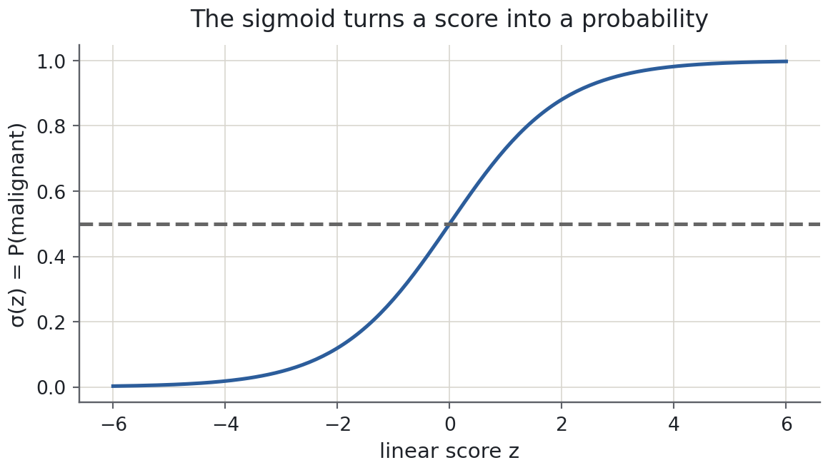
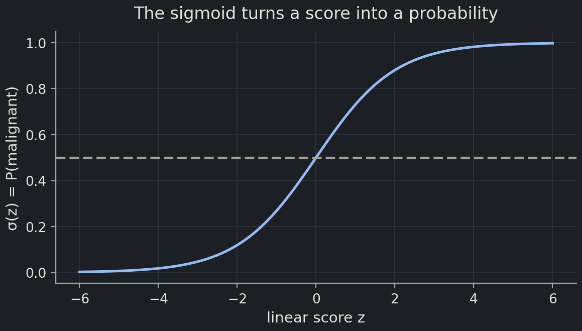
The simplest classifier is a linear model in disguise. logistic regressionlogistic regressionA linear model for classification that outputs probabilities through the sigmoid function. computes the same weighted sum as linear regression, \(z = \theta_0 + \theta_1 x_1 + \dots + \theta_p x_p\), and then squashes it through the sigmoid functionsigmoid functionThe S-shaped function σ(z) = 1/(1+e^(−z)) that squashes any number into (0, 1). function
\[
\sigma(z) = \frac{1}{1 + e^{-z}},
\]
which maps any real number to a value between 0 and 1 that we read as the probability of the positive class. A large positive \(z\) means “confidently malignant”, a large negative \(z\) “confidently benign”, and \(z = 0\) sits exactly on the fence at a probability of 0.5.
import matplotlib.pyplot as pltz = np.linspace(-6, 6, 200)fig, ax = plt.subplots(figsize=(6, 3.4))ax.plot(z, 1/ (1+ np.exp(-z)))ax.axhline(0.5, linestyle="--", color="0.4")ax.set(xlabel="linear score z", ylabel="σ(z) = P(malignant)", title="The sigmoid turns a score into a probability")plt.show()
Training finds the \(\theta\) that makes these probabilities agree with the labels, by minimising the log loss rather than the squared error. You do not need the formula to use the model; the maths corner below has it.
Maths corner
Logistic regression is a generalised linear model: \(\log \frac{p}{1-p} = \theta^\top x\), so the log-odds are linear in the features. The loss is the negative log-likelihood of a Bernoulli model, \(-\sum_i \left[ y_i \log p_i + (1 - y_i)\log(1 - p_i) \right]\), which is convex, so gradient descent finds the global minimum. Its gradient has the same shape as the one you derived for MSE in episode 2.2: \(X^\top (p - y)\).
Because the model penalises large coefficients by default (scikit-learn’s LogisticRegression applies an L2 penalty, like ridge), the features must be on comparable scales. We put a StandardScaler in front, inside a pipelinepipelineA chain of preprocessing steps and a model that is fitted and applied as one unit.; episode 2.6 explains why this matters and why it must be inside the pipeline.
About 96.5% accuracy against a baseline of 63%. The model clearly improves on the baseline, but predict hides something: the model first estimates probabilities, then turns them into classes.
predict simply applies a decision thresholddecision thresholdThe probability above which a classifier predicts the positive class; 0.5 is only a default. of 0.5 to those probabilities. That 0.5 is a default, not a law, and we will move it later.
Seeing the decision boundary
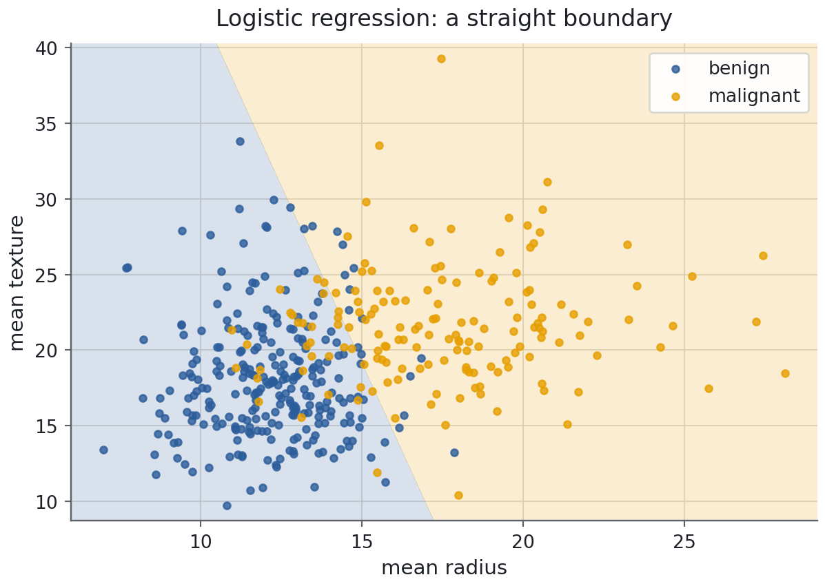
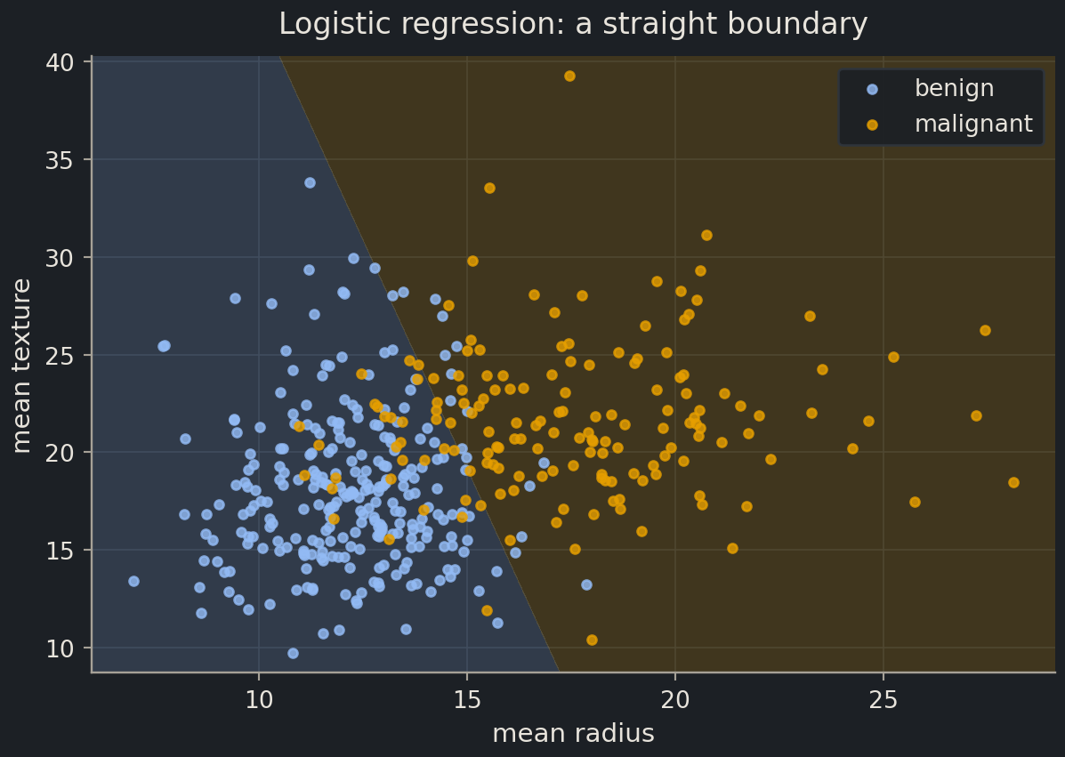
With 30 features the model’s boundary lives in 30 dimensions. To see one, train on two features only, mean radius and mean texture, and shade the plane by the predicted class.
The boundary is a straight line, because the score \(z\) is linear in the features: every point on one side is called malignant, every point on the other benign, and the probability rises smoothly as you move away from the line. The misclassified points near the line are tumours whose size and texture alone cannot settle; with all 30 features the model does much better.
For programmers
predict returns a class, predict_proba returns the probabilities, and decision_function returns the raw score \(z\). The threshold is applied at prediction time, so it is a deployment knob: never bake “0.5” into downstream code; pass the probabilities along and let the application decide.
k-nearest neighbours: a boundary that follows the data
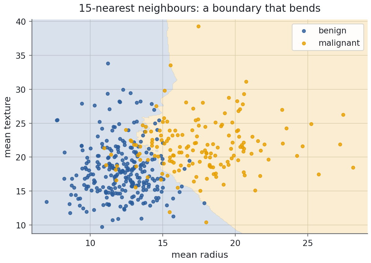
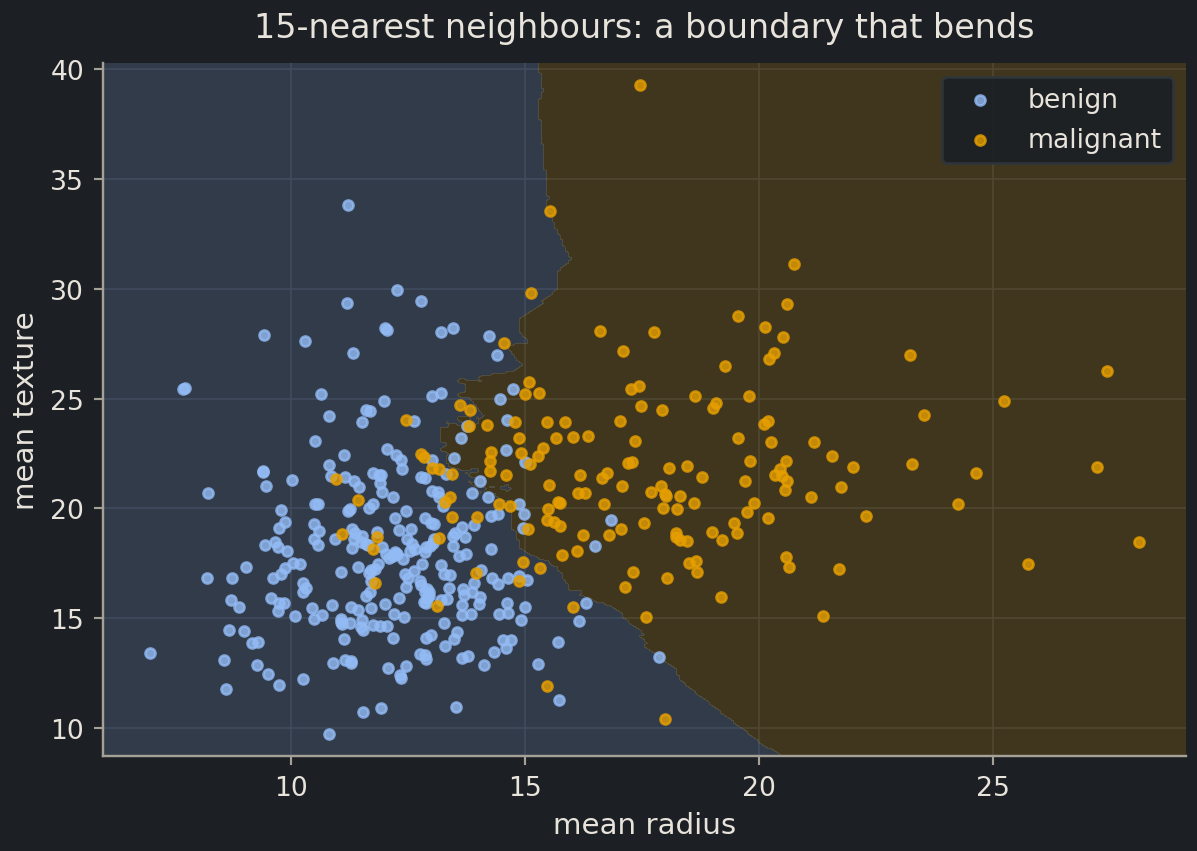
A completely different idea: to classify a new tumour, find the \(k\) most similar tumours in the training set and take a vote. That is k-nearest neighbours (kNN)k-nearest neighbours (kNN)Predicting a sample from the k most similar training samples.. It has no parameters to train and no equation for the boundary; the boundary is whatever the training points make it.
from sklearn.neighbors import KNeighborsClassifierknn2 = make_pipeline(StandardScaler(), KNeighborsClassifier(n_neighbors=15)).fit(X_train[two], y_train)fig, ax = plt.subplots(figsize=(6.2, 4.4))DecisionBoundaryDisplay.from_estimator( knn2, X_train[two], response_method="predict", plot_method="contourf", levels=[-0.5, 0.5, 1.5], grid_resolution=400, cmap=class_cmap, alpha=0.18, ax=ax,)for label, name in [(0, "benign"), (1, "malignant")]: sub = X_train[y_train == label] ax.scatter(sub["mean radius"], sub["mean texture"], s=14, alpha=0.8, color=class_colors[label], label=name)ax.set(xlabel="mean radius", ylabel="mean texture", title="15-nearest neighbours: a boundary that bends")ax.legend()plt.show()
The number of neighbours \(k\) is a hyperparameterhyperparameterA setting chosen before training, such as the number of neighbours in kNN or the strength of regularisation., and it controls exactly the flexibility you studied in episode 2.4.
Predict before you run
Before running the next cell: what training accuracy will a 1-nearest-neighbour classifier have? And will its test accuracy be higher or lower than with \(k = 15\)?
rows = []for k in [1, 5, 15, 51]: model = make_pipeline(StandardScaler(), KNeighborsClassifier(n_neighbors=k)).fit(X_train[two], y_train) rows.append({"k": k, "train accuracy": model.score(X_train[two], y_train), "test accuracy": model.score(X_test[two], y_test)})pd.DataFrame(rows).round(3)
index
k
train accuracy
test accuracy
0
1
1.000
0.874
1
5
0.904
0.902
2
15
0.899
0.895
3
51
0.908
0.916
With \(k = 1\) every training point is its own nearest neighbour, so the training accuracy is a perfect 1.0, and the test accuracy is the worst of the four: the textbook overfitting signature. Larger \(k\) smooths the boundary. Because kNN decides by distance, it is also the model most sensitive to feature scaling, which is why the scaler is in the pipeline.
Reading a classifier properly
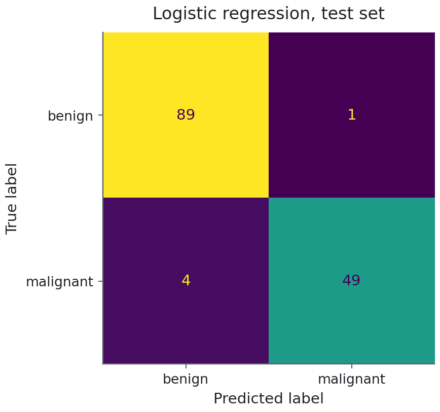
Accuracy compresses four numbers into one. The four numbers are the confusion matrixconfusion matrixA table counting true/false positives and negatives., and they are where every other metric comes from.
from sklearn.metrics import ConfusionMatrixDisplayfig, ax = plt.subplots(figsize=(4.6, 4.2))ConfusionMatrixDisplay.from_estimator(logreg, X_test, y_test, display_labels=["benign", "malignant"], ax=ax, colorbar=False)ax.grid(False)ax.set(title="Logistic regression, test set")plt.show()
Read it in medical language. Rows are the truth, columns the prediction:
True positives (bottom right): malignant tumours called malignant. 49.
False negatives (bottom left): malignant tumours called benign. 4. The dangerous cell: missed cancers.
False positives (top right): benign tumours called malignant. 1. A frightened patient and an unnecessary biopsy.
True negatives (top left): benign called benign. 89.
From these four cells:
Metric
Formula
Question it answers
accuracy
\((TP + TN) / n\)
how often is the model right overall?
precisionprecisionOf the samples predicted positive, the fraction that really are positive.
\(TP / (TP + FP)\)
when it says malignant, how often is it right?
recallrecallOf the truly positive samples, the fraction the model finds.
\(TP / (TP + FN)\)
of the malignant tumours, how many did it find?
F1F1 scoreThe harmonic mean of precision and recall; high only when both are high.
Recall for the malignant class is what a clinician calls sensitivity; recall for the benign class is specificity. A screening test wants high sensitivity (miss nothing), and accepts a lower precision (some false alarms) because the follow-up test will sort them out. A confirmatory test wants the opposite. The same model can serve both roles: only the threshold changes.
Across all thresholds: ROC and precision–recall curves
The confusion matrix is a snapshot at one threshold. Two curves show the model at every threshold at once.
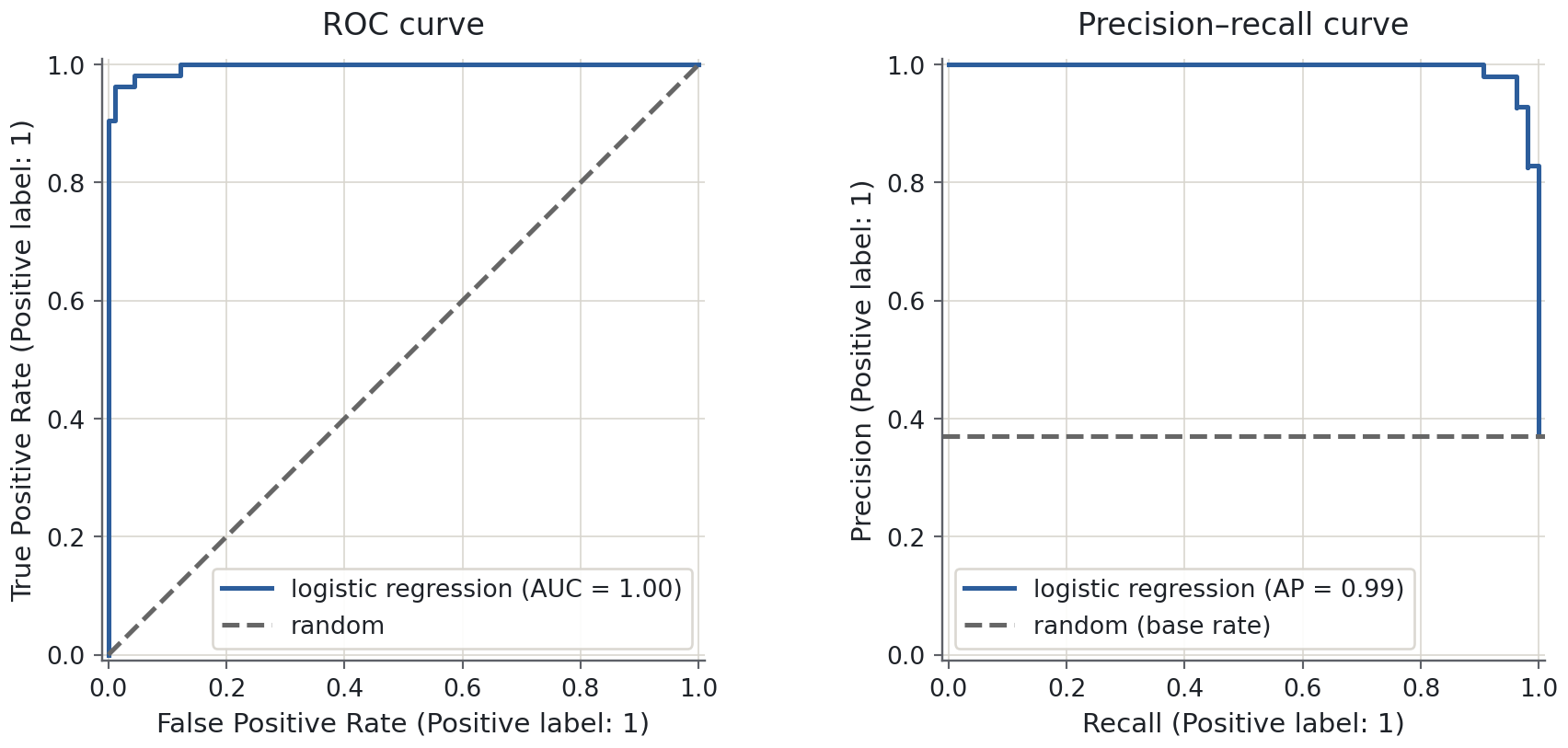
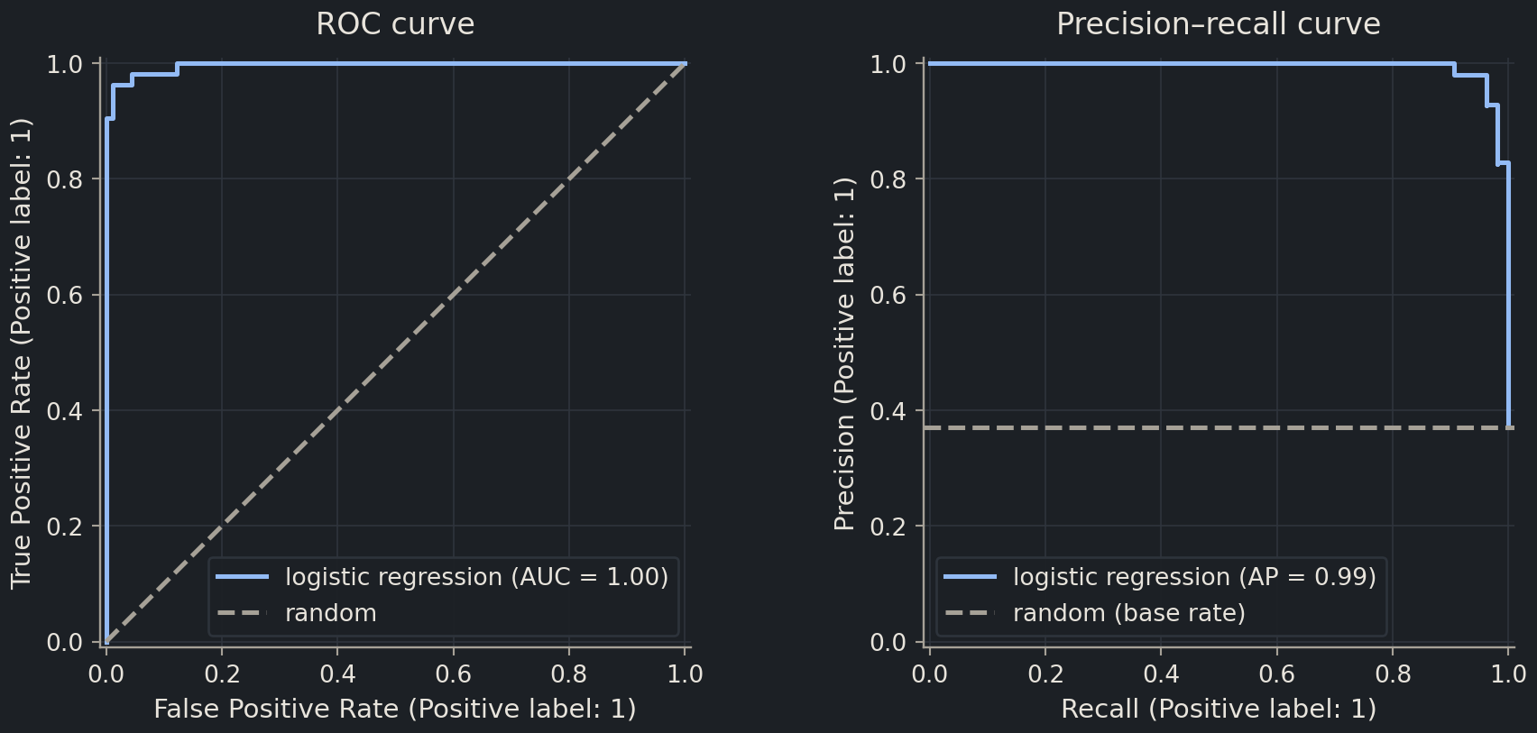
The ROC curveROC curve and AUCA curve of true-positive rate against false-positive rate across thresholds; AUC is the area under it. plots the true-positive rate (recall) against the false-positive rate as the threshold slides from 1 down to 0. A random model follows the diagonal; a perfect one goes straight up the left edge. The area under it, the AUC, summarises how well the model ranks malignant above benign: 0.5 is random, 1.0 is perfect.
The precision–recall curveprecision–recall curvePrecision against recall across thresholds; more informative than ROC when positives are rare. plots precision against recall over the same thresholds. Its baseline is not the diagonal but the base rate of the positive class, the horizontal dashed line, which is where a random model sits. The two curves answer different questions. ROC ignores how rare the positives are, so it looks flattering when they are rare; the precision–recall curve does not, which is why it is the one to show when the positive class is a small minority.
Common mistake
AUC says nothing about the threshold you will use
A model with AUC 0.99 can still be useless at the default threshold if its probabilities are shifted, and two models with the same AUC can behave very differently at the operating point you care about. AUC compares rankings; the confusion matrix at your threshold is what the user of the model experiences.
Choosing the threshold
Suppose missing a malignant tumour is far worse than a false alarm. Then you lower the threshold: call a tumour malignant at a probability of, say, 0.2 instead of 0.5. Recall cannot decrease, and there may be more false alarms; precision often falls, though it need not change monotonically. Nothing is retrained; you are just reading the same probabilities differently.
from sklearn.metrics import precision_score, recall_scorerows = []for t in [0.5, 0.3, 0.2, 0.1, 0.05]: pred = (probs >= t).astype(int) rows.append({"threshold": t, "recall (malignant)": recall_score(y_test, pred), "precision (malignant)": precision_score(y_test, pred)})pd.DataFrame(rows).round(3)
index
threshold
recall (malignant)
precision (malignant)
0
0.50
0.925
0.980
1
0.30
0.962
0.981
2
0.20
0.962
0.944
3
0.10
0.981
0.897
4
0.05
1.000
0.828
On this test set, a threshold of 0.1 still misses one malignant tumour; 0.05 catches all 53, with 11 false alarms. This table illustrates the trade-off, but choosing a threshold from it would use the test set for tuning. Choose the threshold using training or validation data, as in the exercise below, then evaluate that fixed choice on a held-out test set. The right trade-off depends on the cost of each kind of mistake and the people who will act on the predictions.
When the class you want is rare
The breast cancer data is nearly balanced, 37% malignant. Scientific data usually is not. In a high-throughput screen a few compounds in a thousand are active; in a patient cohort most people do not have the disease. This is class imbalanceclass imbalanceWhen one class is much rarer than the other, so accuracy becomes misleading., and it breaks accuracy completely.
Chemist's corner
In a typical primary screen about 1% of compounds, often fewer, show activity. A model that predicts “inactive” for every compound is therefore 99% accurate and finds nothing. What a medicinal chemist wants is recall of the actives at a manageable number of false positives, because every predicted active will be bought or synthesised and tested. The precision–recall curve and the number of actives found in the top-ranked \(N\) compounds are the metrics that match that workflow; accuracy and even ROC-AUC are not.
To see it, simulate a screen: 8,000 compounds with ten descriptor-like features, of which 1% are active.
from sklearn.datasets import make_classificationX_scr, y_scr = make_classification( n_samples=8000, n_features=10, n_informative=4, n_redundant=2, weights=[0.99, 0.01], class_sep=0.9, flip_y=0, random_state=42,)Xs_train, Xs_test, ys_train, ys_test = train_test_split(X_scr, y_scr, test_size=0.3, random_state=42, stratify=y_scr)print(f"actives in the test set: {ys_test.sum()} of {len(ys_test)}")
The do-nothing baseline has 99% accuracy and finds zero actives. Accuracy is meaningless here.
The ordinary model is slightly more accurate and finds only a handful of actives: at the 0.5 threshold it almost never dares to call anything active, because being wrong about a rare class is cheap in the loss.
class_weight="balanced" tells the model to weight each active as heavily as the 99 inactives it is outnumbered by. Recall jumps, accuracy falls, and the false alarms multiply. For a screen that is often the right trade: those false alarms are the compounds you will test next.
Reporting the precision–recall curve rather than the ROC curve, stratifying every split, and choosing the threshold from the cost of a false alarm are the three habits that make a model on rare events honest.
Note
A note on calibration
A probability of 0.8 should mean “about 80 of 100 such tumours are malignant”. When that holds the model is well calibratedcalibrationWhether predicted probabilities match observed frequencies: of samples given 0.8, about 80% should be positive.. Good ranking (high AUC) does not guarantee it: kNN with small \(k\) outputs only a few distinct probabilities, and class weighting deliberately distorts them. scikit-learn’s CalibrationDisplay.from_estimator draws the check; CalibratedClassifierCV repairs it. Calibration matters whenever you will act on the probability itself, for example when ranking compounds to buy under a budget.
Discussion
A paper reports “our toxicity classifier reaches 97% accuracy”. The dataset has 4% toxic compounds. What is the first number you would ask for, and what would convince you the model is useful to a chemist?
Exercises
Exercise★☆☆
Metrics from a confusion matrix
A classifier for signal peptides is tested on 200 proteins: 40 contain a signal peptide. It predicts “signal peptide” for 50 proteins, of which 32 are correct. Without code, fill in the confusion matrix and compute accuracy, precision, recall and F1 for the signal-peptide class.
Note how a respectable 87% accuracy hides a precision of only 0.64: more than a third of the predicted signal peptides are wrong. The majority baseline (“no signal peptide” for everyone) would score 160 / 200 = 0.80 accuracy and find none.
Exercise★★☆
A threshold for a screening test
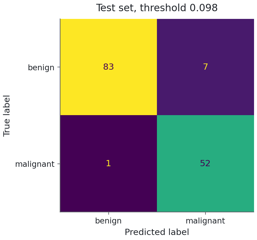
Generate out-of-fold probabilities on X_train with cross_val_predict, so each training tumour is predicted by a pipeline fitted without that tumour. Find the highest threshold at which the out-of-fold recall for malignant tumours is at least 0.98, and report the precision there. Then apply that fixed threshold to probs from the test set and draw its confusion matrix. (Hint: precision_recall_curve from sklearn.metrics returns the thresholds.)
SolutionShow solutionHide solution
from sklearn.metrics import precision_recall_curvefrom sklearn.model_selection import StratifiedKFold, cross_val_predictthreshold_cv = StratifiedKFold(n_splits=5, shuffle=True, random_state=42)train_probs = cross_val_predict( logreg, X_train, y_train, cv=threshold_cv, method="predict_proba")[:, 1]precision, recall, thresholds = precision_recall_curve(y_train, train_probs)# precision/recall have one more entry than thresholds; drop the last pointok = recall[:-1] >=0.98best = thresholds[ok].max()i = np.where(thresholds == best)[0][0]print(f"threshold {best:.3f}: out-of-fold recall {recall[i]:.3f}, precision {precision[i]:.3f}")
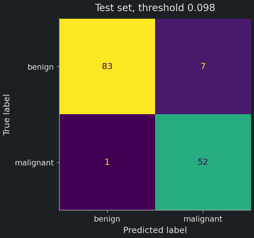
precision_recall_curve evaluates every distinct probability as a threshold, so it finds the exact operating point on these predictions rather than one on a coarse grid. The highest threshold satisfying the recall target calls the fewest tumours positive among the eligible choices; it does not guarantee the highest precision. Here the training out-of-fold threshold is about 0.098. Applied unchanged to the test set, it finds 52 of 53 malignancies with seven false alarms: recall about 0.981 and precision about 0.881. The target recall is a training-data choice, not a guarantee for future samples.
Exercise★★★
kNN against logistic regression, honestly
Compare make_pipeline(StandardScaler(), KNeighborsClassifier(n_neighbors=k)) for \(k \in \{1, 5, 15, 51\}\) against the logistic regression pipeline on all 30 features, using 10-fold stratified cross-validation (StratifiedKFold(n_splits=10, shuffle=True, random_state=42)) on the training set and the scoring "roc_auc". Which model wins, how sure are you, and what does the \(k = 1\) result tell you about cross-validation versus the training score you saw earlier?
Logistic regression is at least as good as the best kNN and more stable across folds, which is typical for a dataset of this size with informative, roughly linear features. \(k = 1\) is clearly worst even though its training accuracy was perfect: cross-validation exposes what the training score hid. The standard deviations tell you how much the ranking can move between folds; differences smaller than about one standard deviation are not worth arguing about. StratifiedKFold keeps the malignant fraction equal in every fold, which matters for AUC on small folds.
Where this is going
Classification in this course mostly means finding rare positives: active compounds in a screen, binding poses that are correct, proteins with a given function, cells of a given type. Chapter 6 (QSAR) uses exactly the metrics of this episode, precision–recall curves and actives-found-in-top-N, on fingerprint features with scaffold splits in place of the random split used here. Chapter 10 does the same for sequences with sequence-identity splits. The threshold discussion returns in Chapter 14, where a generative model proposes compounds and a classifier decides which to make: there, the cost of a false positive is a synthesis that fails, and the threshold is chosen from a budget.
Key points
Logistic regression is a linear model whose output passes through the sigmoid to give a probability; the class is a threshold on that probability.
Always compare against DummyClassifier; on imbalanced data a useless model can have impressive accuracy.
The confusion matrix is the ground truth. Precision, recall and F1 are read from it; report them for the class you care about.
ROC/AUC measures ranking across all thresholds; the precision–recall curve is the honest picture when positives are rare.
The threshold is a decision, not a constant: move it to trade recall against precision.