What do I actually do with a new dataset before I model anything?
What is logS, and why do chemists model the logarithm of solubility rather than solubility itself?
Which of the descriptors in the ESOL file are related to solubility, and how strongly?
What you will be able to do
Load the ESOL dataset with the local-file-then-URL idiom and check its shape, types and missing values.
Describe the distribution of a target variable and of each descriptor with histograms and describe().
Relate descriptors to the target with coloured scatter plots and a correlation heatmap.
Find the most and least soluble compounds, check for duplicate molecules, and explain what a SMILES string is.
State the modelling question that Chapter 2 answers, and what the EDA suggests about it.
A medicinal chemist has just made a compound that binds its target beautifully in the assay. Then it fails: it will not dissolve in water, so it never reaches the bloodstream of the animal it is dosed to. Poor aqueous solubility is one of the most common reasons a promising compound goes no further, and it would be enormously useful to predict it before the compound is made. That is the question behind this episode and behind Chapter 2: can we predict how soluble a molecule is from a few numbers that describe its structure?
Before anyone fits a model, a careful scientist spends an hour looking at the data. That hour is exploratory data analysisexploratory data analysis (EDA)Looking at distributions, relationships and oddities in the data before modelling. (EDA), and it has a checklist that is nearly the same for every table you will ever meet: shape, types, missing values, the distribution of the thing you want to predict, the distribution of each input, how the inputs relate to the target and to each other, outliers, duplicates. This episode runs that checklist on a classic dataset, using everything from episode 1.3 and episode 1.4.
Biologist's corner
Aqueous solubility is how much of a compound dissolves in water at equilibrium, here expressed as a concentration in moles per litre. For a drug taken by mouth it is a gatekeeper: a tablet has to dissolve in the fluid of the gut before anything can be absorbed across the gut wall, and a compound that stays as a solid passes straight through. In the laboratory it decides whether you can make a stock solution at a useful concentration without a solvent that harms your cells. Formulation, the craft of turning a compound into a dosable medicine, has tricks to help (salts, particle size, carriers), but every trick costs time and money, so projects try hard to avoid insoluble compounds in the first place.
The data
The ESOL dataset was published by Delaney in 2004: 1,128 small organic molecules with a measured solubility, each described by a few simple numbers that can be computed from the structure alone. The file is not bundled with the course, so we load it with an idiom you will see again in Chapter 2: use the local copy if it exists, otherwise read it straight from the URL.
from pathlib import Pathimport matplotlib.pyplot as pltfrom matplotlib.ticker import MaxNLocatorimport pandas as pdimport seaborn as snsESOL_URL ="https://deepchemdata.s3-us-west-1.amazonaws.com/datasets/delaney-processed.csv"path = Path("data/esol.csv")esol = pd.read_csv(path if path.exists() else ESOL_URL)esol.shape
(1128, 10)
1,128 rows and 10 columns. Column names first, because they are long and we will refer to them often.
esol.columns.tolist()
['Compound ID',
 'ESOL predicted log solubility in mols per litre',
 'Minimum Degree',
 'Molecular Weight',
 'Number of H-Bond Donors',
 'Number of Rings',
 'Number of Rotatable Bonds',
 'Polar Surface Area',
 'measured log solubility in mols per litre',
 'smiles']
The last-but-one column is the measurement we want to predict, the labellabelThe quantity you want to predict for each sample; the vector y.; in this course we call it the target. Give it a short name so that the long string appears once:
target ="measured log solubility in mols per litre"esol[["Compound ID", "Molecular Weight", "Number of Rings", target]].head()
index
Compound ID
Molecular Weight
Number of Rings
measured log solubility in mols per litre
0
Amigdalin
457.432
3
-0.77
1
Fenfuram
201.225
2
-3.30
2
citral
152.237
0
-2.06
3
Picene
278.354
5
-7.87
4
Thiophene
84.143
1
-1.33
The other numeric columns are molecular descriptorsmolecular descriptorA number computed from a molecule’s structure, such as molecular weight or polar surface area.: numbers computed from the molecular structure, which will be the model’s featuresfeatureAn input variable describing a sample; one column of the X matrix.. One column is special, ESOL predicted log solubility in mols per litre: it is the output of Delaney’s own model, not a property of the molecule, and we will keep it out of the descriptor set. Minimum Degree is a graph-theoretic quantity that is 1 for all but 68 of the molecules, so it carries almost no information and we will drop it too.
Types and missing values next, exactly as in episode 1.3.
esol.dtypes
Compound ID                                            str
ESOL predicted log solubility in mols per litre    float64
Minimum Degree                                       int64
Molecular Weight                                   float64
Number of H-Bond Donors                              int64
Number of Rings                                      int64
Number of Rotatable Bonds                            int64
Polar Surface Area                                 float64
measured log solubility in mols per litre          float64
smiles                                                 str
dtype: object
esol.isna().sum().sum()
np.int64(0)
Two text columns (Compound ID and smiles), eight numeric ones, and not a single missing value. That is unusual for real data and worth noting: this file has already been cleaned. Do not expect it elsewhere.
What is logS?
The target is called log solubility: it is \(\log_{10}\) of the solubility \(S\) in mol/L, written logSlogSThe base-10 logarithm of aqueous solubility in mol/L; the ESOL target.. A value of −3 means \(S = 10^{-3}\) mol/L, one millimole per litre; a value of −6 means a micromole per litre, a thousand times less soluble. Each unit of logS is a factor of ten in solubility.
esol[target].describe().round(2)
count    1128.00
mean       -3.05
std         2.10
min       -11.60
25%        -4.32
50%        -2.86
75%        -1.60
max         1.58
Name: measured log solubility in mols per litre, dtype: float64
The median compound has logS ≈ −2.9, about one millimole per litre. The range runs from +1.58 (acetamide, so soluble that it dissolves at nearly 40 mol/L) down to −11.6, a difference of more than thirteen orders of magnitude.
Chemist's corner
Why does everyone model logS rather than \(S\) itself? Three reasons. First, the range: \(S\) in this file spans from \(10^{-11.6}\) to \(10^{1.6}\) mol/L. A straight line fitted to \(S\) would spend all its effort on the dozen most soluble compounds, because their values are millions of times larger than everyone else’s, and would treat the difference between 1 µM and 1 nM as zero. Second, errors in log units are relative errors, which is how you think at the bench: being out by one log unit means a factor of ten, whether the compound is at 1 M or 1 µM. Third, the physics: solubility is governed by free energies of solvation and crystal packing, and free energy is proportional to the logarithm of a concentration, so the quantities that structure actually controls are additive on the log scale. The same argument applies to IC₅₀ (hence pIC₅₀), partition coefficients (logP) and rate constants.
Deep diveLogarithms, factors and the geometric meanShow the mathsHide the maths
\(\log_{10} S\) is the power to which 10 must be raised to give \(S\): \(\log_{10} 10^{-3} = -3\). Adding 1 to logS multiplies \(S\) by 10; adding 0.3 multiplies it by \(10^{0.3} \approx 2\). Differences on the log scale are therefore ratios on the original scale.
Averages behave differently on the two scales. The arithmetic mean of logS in this dataset is −3.05, which corresponds to \(10^{-3.05} \approx 0.9\) mmol/L. The arithmetic mean of \(S\) itself is 0.39 mol/L, four hundred times larger, because a few very soluble compounds dominate the sum. The quantity \(10^{\text{mean}(\log S)}\) is the geometric mean, \(\left(\prod_i S_i\right)^{1/n}\), and it is the sensible “typical” solubility when values spread over many orders of magnitude. The same is true of the log transformlog transformTaking the logarithm of a quantity that spans orders of magnitude, so that ratios become differences. of any right-skewed positive quantity: concentrations, counts, incomes, gene expression levels.
The distribution of the target
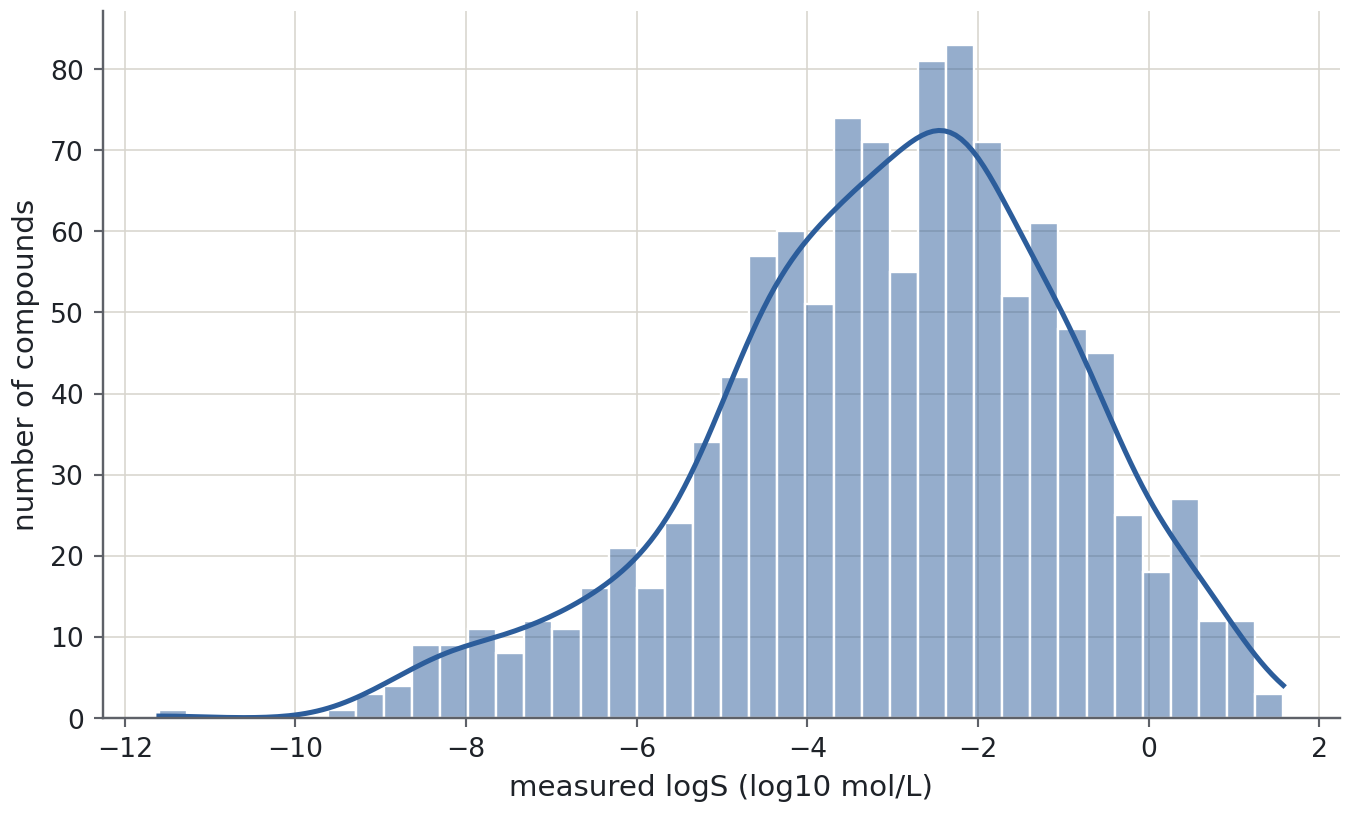
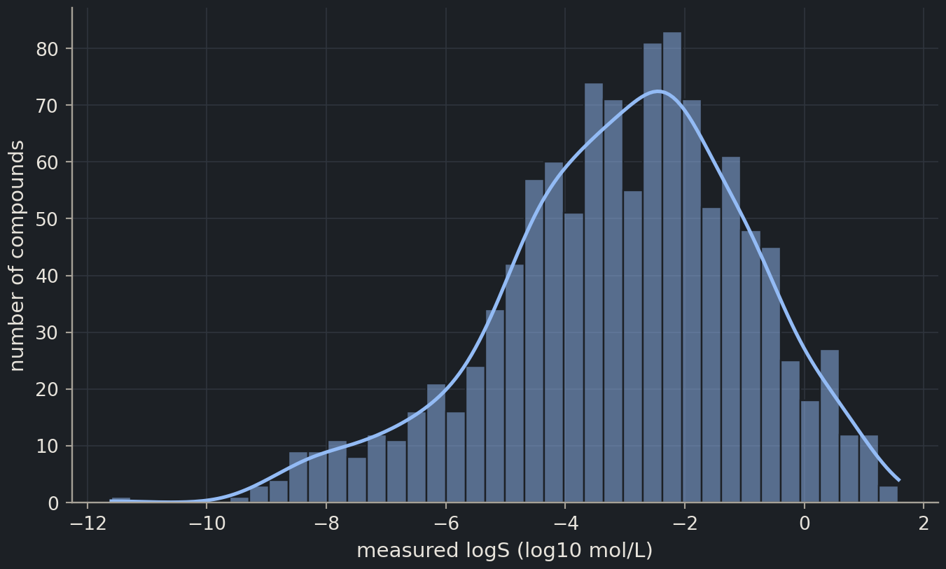
The first picture is always the target’s histogramhistogramBars counting how many values fall into each interval (bin) of a variable.. You are looking for the shape (one peak or several?), the width, and the tails.
One broad peak, roughly bell-shaped on the log scale, which is itself a sign that the log transform was the right choice. The left tail is long: a few dozen compounds below −7 that are practically insoluble. Keep them in mind; models tend to struggle at the ends of a distribution.
The descriptors
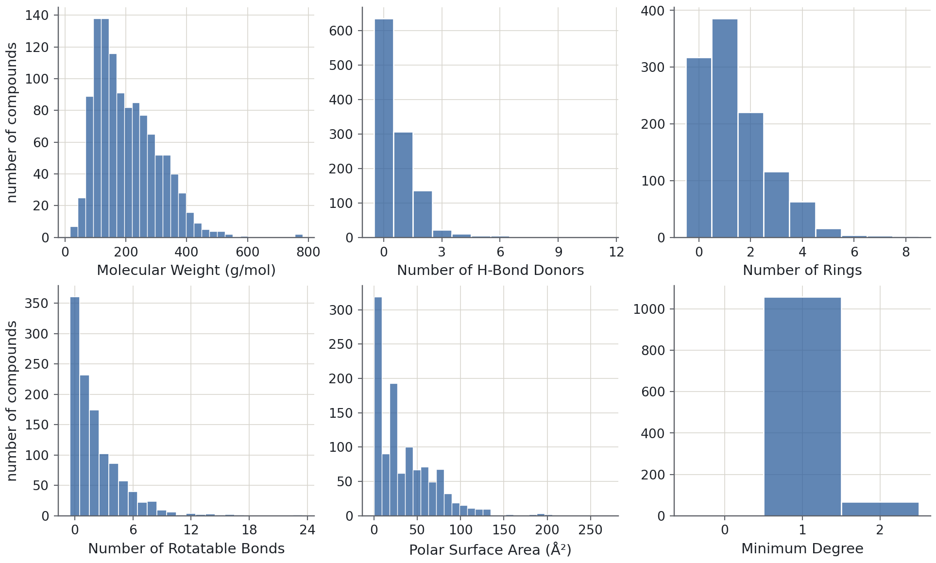
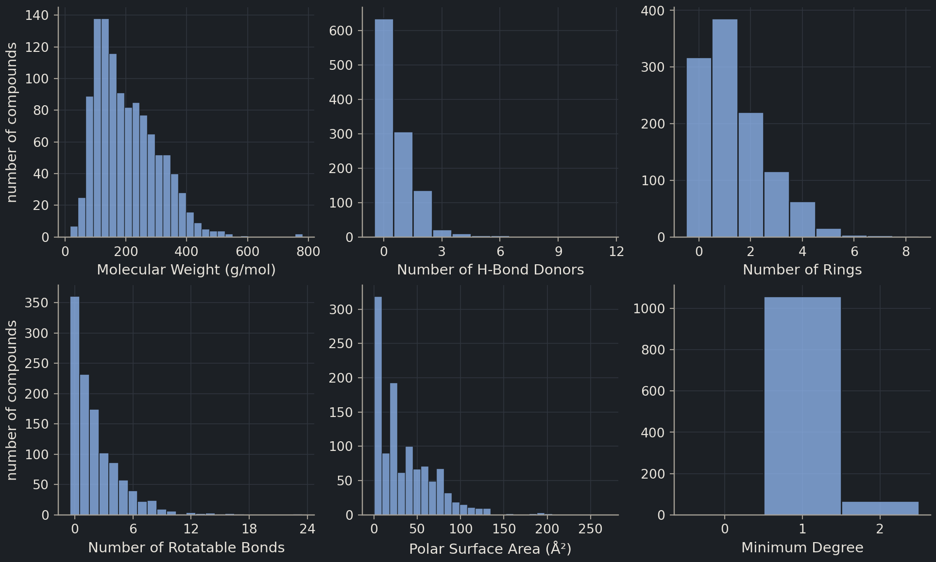
Now the inputs. Before dropping Minimum Degree, inspect all six structural descriptors in a 2 × 3 grid of histograms.
descriptors = ["Molecular Weight","Number of H-Bond Donors","Number of Rings","Number of Rotatable Bonds","Polar Surface Area","Minimum Degree",]esol[descriptors].describe().round(1)
index
Molecular Weight
Number of H-Bond Donors
Number of Rings
Number of Rotatable Bonds
Polar Surface Area
Minimum Degree
count
1128.0
1128.0
1128.0
1128.0
1128.0
1128.0
mean
203.9
0.7
1.4
2.2
34.9
1.1
std
102.7
1.1
1.3
2.6
35.4
0.2
min
16.0
0.0
0.0
0.0
0.0
0.0
25%
121.2
0.0
0.0
0.0
0.0
1.0
50%
182.2
0.0
1.0
1.0
26.3
1.0
75%
270.4
1.0
2.0
3.0
55.4
1.0
max
780.9
11.0
8.0
23.0
268.7
2.0
units = {"Molecular Weight": "g/mol", "Polar Surface Area": "Ų"}fig, axes = plt.subplots(2, 3, figsize=(10, 6))for ax, col inzip(axes.flat, descriptors): is_count = col notin units sns.histplot(data=esol, x=col, bins=30, discrete=is_count, ax=ax)if is_count: ax.xaxis.set_major_locator(MaxNLocator(nbins=5, integer=True)) ax.set(xlabel=f"{col} ({units[col]})"if col in units else col, ylabel="")axes[0, 0].set(ylabel="number of compounds")axes[1, 0].set(ylabel="number of compounds")plt.show()
Two kinds of descriptor appear. Molecular weight and polar surface area are continuous and right-skewed. The counts (donors, rings, rotatable bonds) are integers, mostly small, with a few compounds far out on the right; discrete=True centres one bin on each integer. Minimum Degree has one dominant bar at 1 (1,060 compounds), a smaller bar at 2 (67), and one compound at 0. From here on we work with the five informative descriptors.
descriptors = descriptors[:5]
Descriptors against the target
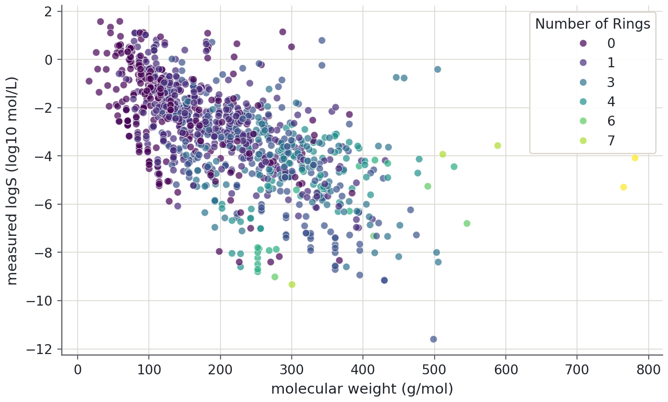
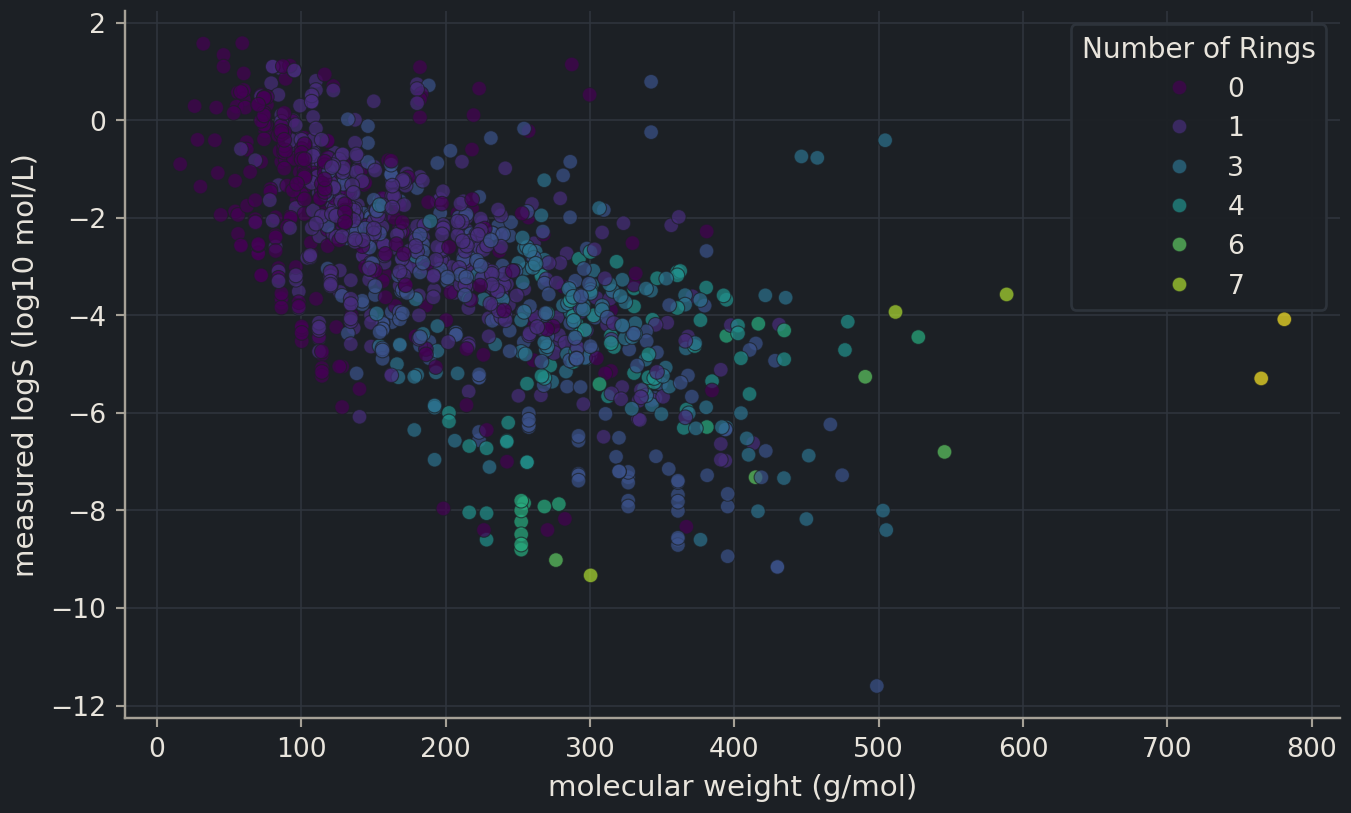
Which descriptors matter? Plot each against logS. Colour carries a third variable; because ring count and donor count are ordered quantities, use the sequential viridis colourmap rather than a categorical palette.
Predict before you run
Before you run the next cell, decide: as molecular weight increases, does logS go up or down? And will the compounds with many rings sit above or below the others at the same weight?
Heavier molecules are less soluble: the cloud slopes down, though it is wide. At the same weight, the yellower points (more rings) tend to sit lower than the purple ones (few rings). (Because the hue column is numeric, seaborn treats colour as a continuous scale and lists only a few representative values in the legend; the full scale runs from 0 to 8 rings.) Rings, particularly aromatic ones, make a molecule flat and rigid and good at packing into a crystal, and they contribute little polarity.
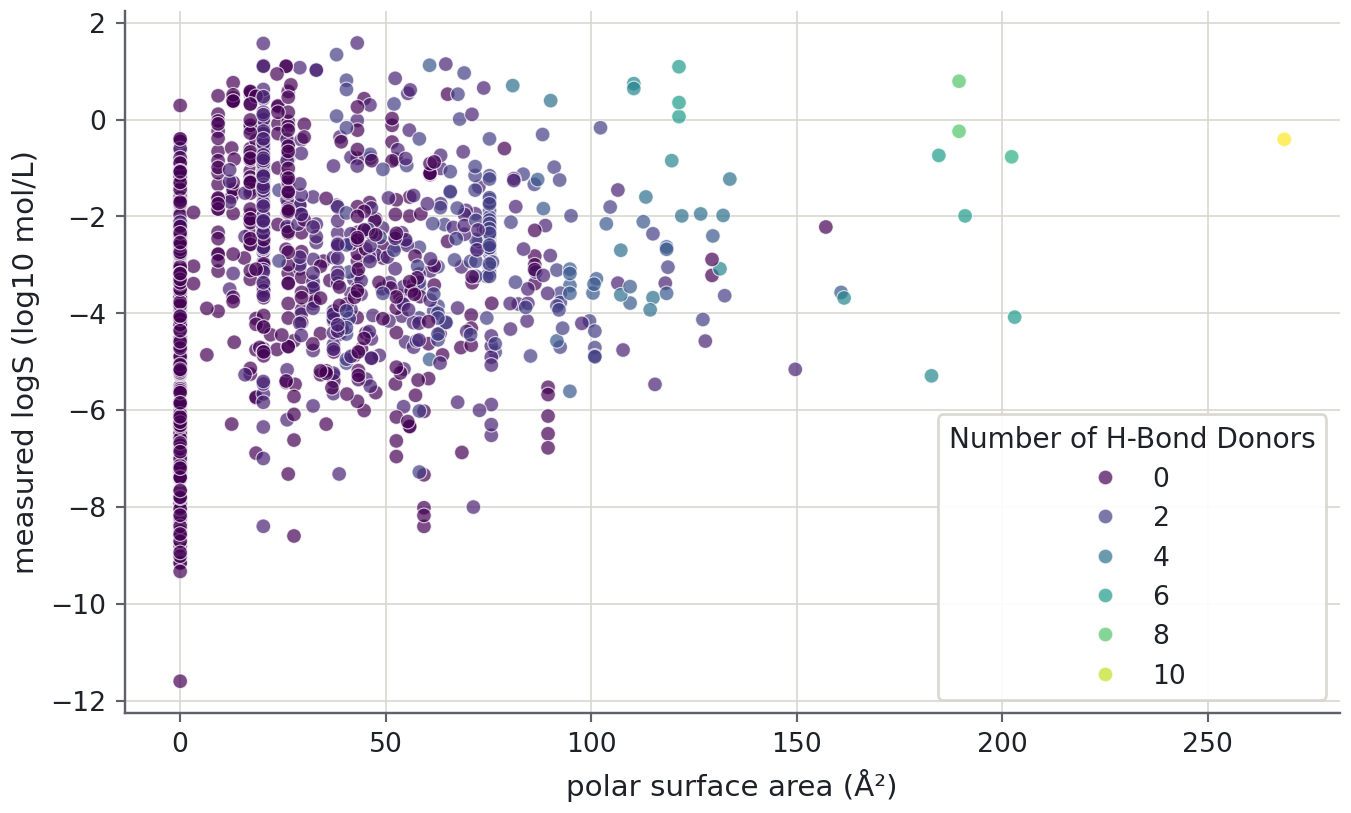
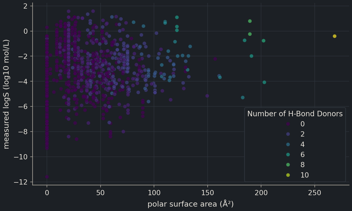
Now polar surface area, coloured by the number of hydrogen-bond donors. Both are measures of how much of the molecule can interact with water.
The relationship is far weaker. Polar molecules are, on average, slightly more soluble, but the band is wide and the most insoluble compounds in the file all have polar surface area near zero without being distinguishable from many soluble ones. Polarity helps; its absence does not condemn a molecule by itself.
Chemist's corner
Nothing in these plots will surprise you: the “general solubility equation” says that logS falls with the melting point and with logP, and both are driven by size, rigidity and lipophilicity. The point of the exercise is different. We are checking what a model could learn from these five numbers alone, with no logP and no melting point. Molecular weight and ring count are standing in for lipophilicity, imperfectly. That is why the linear model in Chapter 2 will reach only about \(R^2 \approx 0.7\), and why Part II spends so much time on better representations of a molecule.
Correlations
A correlation coefficientcorrelation coefficientA number between −1 and 1 measuring how linearly two variables move together. heatmap puts a number on every pairwise relationship, including those between the descriptors themselves. Short labels make the plot readable; rename with a dictionary does that without touching the original table.
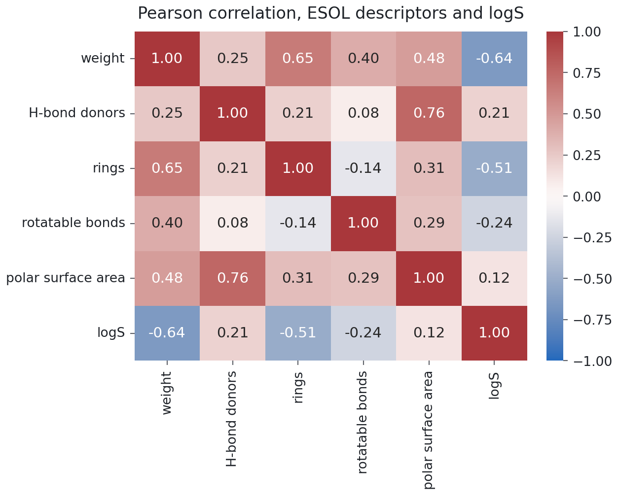
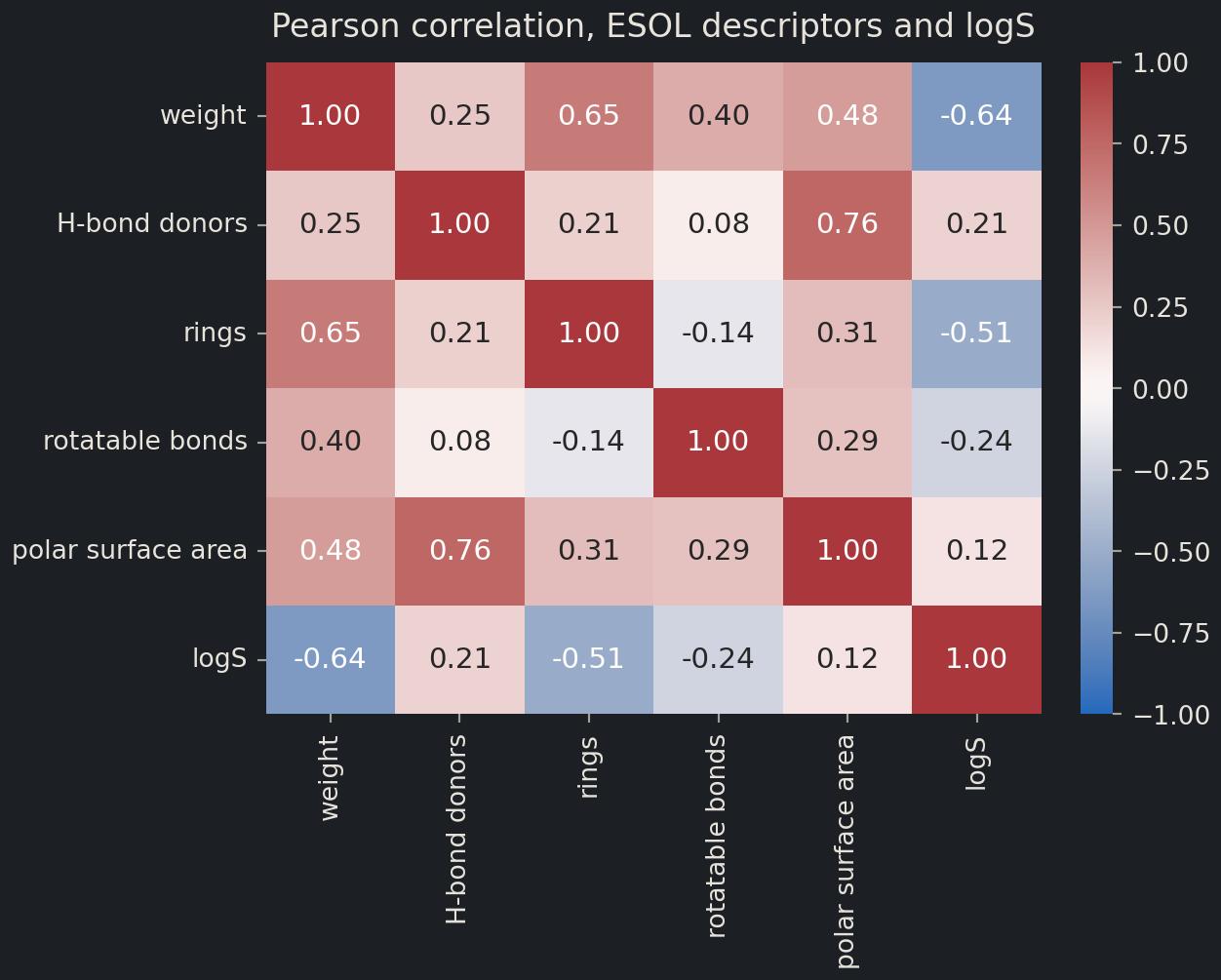
short = {"Molecular Weight": "weight","Number of H-Bond Donors": "H-bond donors","Number of Rings": "rings","Number of Rotatable Bonds": "rotatable bonds","Polar Surface Area": "polar surface area", target: "logS",}corr = esol[descriptors + [target]].rename(columns=short).corr()fig, ax = plt.subplots(figsize=(6.5, 5.2))sns.heatmap(corr, annot=True, fmt=".2f", vmin=-1, vmax=1, cmap="vlag", ax=ax)ax.set(title="Pearson correlation, ESOL descriptors and logS")plt.show()
Read the last row. Molecular weight (−0.64) and ring count (−0.51) are the strongest single predictors of logS; rotatable bonds (−0.24) and the two polarity descriptors (+0.21, +0.12) are weak. Now read the rest. Weight and rings correlate at 0.65, so they partly carry the same information; donors and polar surface area correlate at 0.76, for the obvious reason that donor groups are polar. When two inputs say nearly the same thing, a model gains less from the second than its correlation with the target suggests. You will meet this again under the name collinearity in episode 2.4.
Common mistake
Correlation measures lines
Pearson’s \(r\) measures how well a straight line describes the relationship. A descriptor that affects solubility strongly but non-linearly, say with a threshold, can have a small \(r\) and still be the most useful input for a flexible model. The scatter plots are the check: look for curves, clusters and thresholds that a single number cannot express.
Outliers: the extremes, by name
The ends of the target distribution deserve names. nlargest and nsmallest sort on one column and keep the top rows, and because the file carries a compound name and a structure, you can judge each one.
The most soluble compounds are tiny and polar: acetamide, methanol, methyl hydrazine, glycerol. The least soluble are large, flat molecules made only of carbon and chlorine: a biphenyl with all ten positions chlorinated at the bottom, then coronene and benzo[ghi]perylene, which are sheets of fused benzene rings. Every one of them is chemically reasonable. An outlieroutlierA sample far from the rest; could be an error, a rare case, or the most interesting point. that makes sense is a real observation at the edge of the range, and it stays in. The time to drop a row is when it does not make sense: a logS of +5, a molecular weight of 3, a name that belongs to a different structure.
Duplicates
A dataset assembled from the literature often contains the same molecule twice, sometimes with two different measured values. For a model that is a problem twice over: the duplicate rows get double weight, and if one copy ends up in the training set and the other in the test set, the model is tested on a molecule it has memorised. The duplicateduplicateThe same sample appearing more than once; dangerous when copies land on both sides of a split. check is one line per column.
Each string is a SMILESSMILESA text notation that writes a molecule’s structure as a string of characters. representation of the molecule: atoms as their element symbols, bonds implied by adjacency, branches in parentheses, ring closures as matching digits, aromatic atoms in lower case. CO is methanol and c1ccsc1 is thiophene. Every descriptor in this file was computed from the string in this column, and nothing else about the molecule is stored.
Note
Coming in Chapter 5
For now the smiles column is a label you can read but not compute with. In Chapter 5 you will parse these strings with RDKit, draw the molecules, and compute molecular weight, ring count, polar surface area and hundreds of other descriptors yourself, which is how you will build features for molecules that have no ready-made table. RDKit also answers the duplicate question properly: it converts every string to a canonical form, so that two different spellings of the same molecule become identical. Without it, duplicated() compares spellings, not molecules.
Framing the question
The EDA has told you what a model is up against. The target is well behaved on the log scale but spans thirteen orders of magnitude, with a thin insoluble tail. Two descriptors carry most of the linear signal and are partly redundant with each other; two more carry a weak signal of the opposite sign. The extremes are real molecules, not errors. There are no missing values and no exact duplicates.
So, the question for Chapter 2: given a molecule’s weight, hydrogen-bond donors, rings, rotatable bonds and polar surface area, how accurately can we predict its logS, and how would we know? The first part is a regression problem. The second part, knowing, is what episode 2.3 is about, and the whole chapter begins with episode 2.1, which sets out what “learning from data” means.
Discussion
You have only five descriptors. Based on the plots, which single additional number about a molecule would you most like to have, and why? (Chemists: argue for or against logP. Biologists and mathematicians: what property of the shape of the molecule might matter?)
Exercises
Exercise★☆☆
The strongest descriptor
Without reading the number off the heatmap, compute the correlation of each of the five descriptors with logS and sort the result. Which descriptor is most strongly related to solubility, and in which direction? Is the sign what you expected?
Molecular Weight            -0.640
Number of Rings             -0.512
Number of Rotatable Bonds   -0.244
Polar Surface Area           0.123
Number of H-Bond Donors      0.209
dtype: float64
corrwith correlates every column of the left-hand frame with the single Series on the right. Molecular weight has the largest magnitude, about −0.64: heavier molecules are less soluble. The sign is negative because the dominant effect of adding atoms to a small organic molecule is adding non-polar surface, which water does not like. Ring count comes next, also negative. Note that sort_values() sorts from most negative to most positive, so the strongest negative correlation is at the top and the strongest positive one at the bottom; sort by abs() if you want magnitude only.
Exercise★★☆
Five scatter plots at once
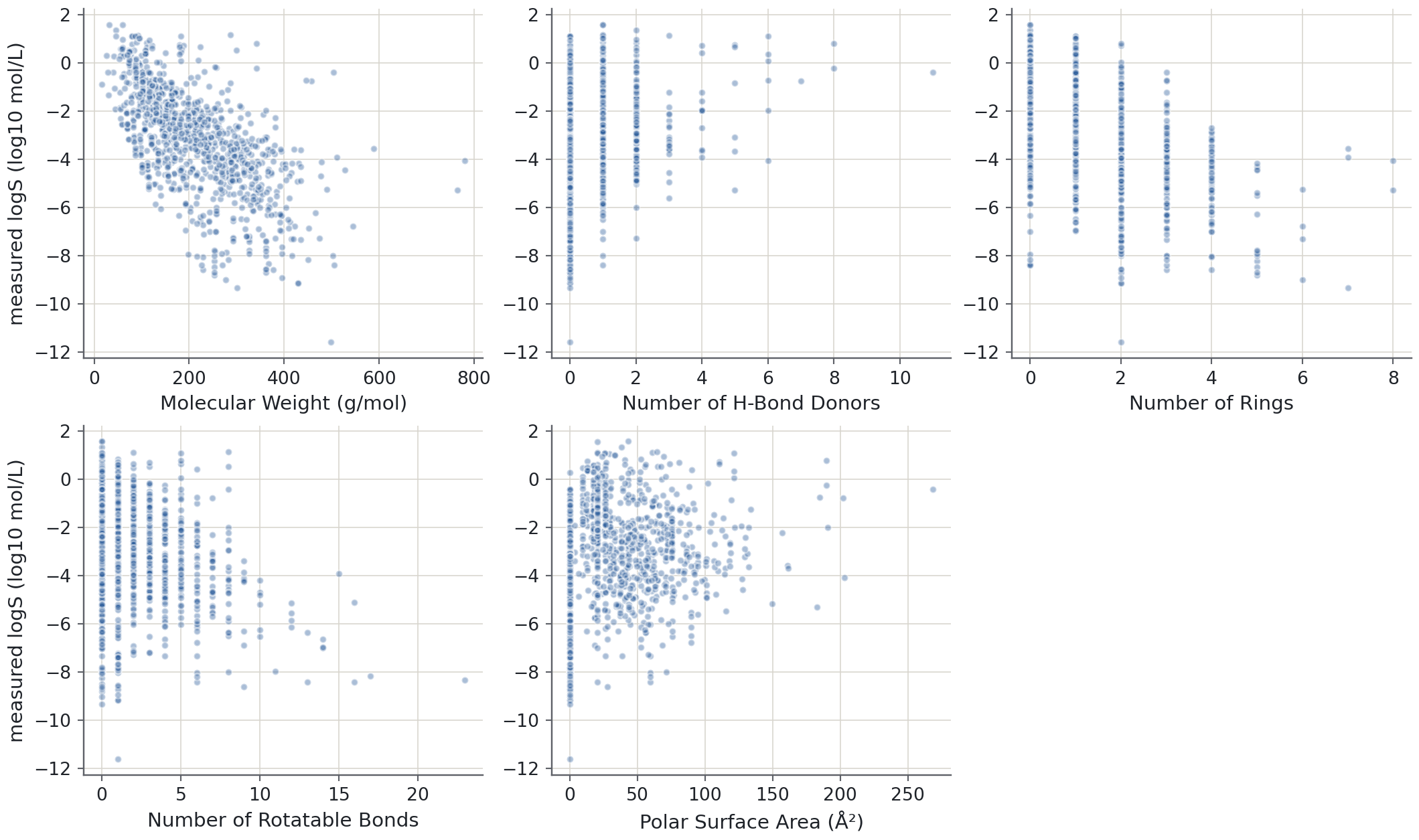
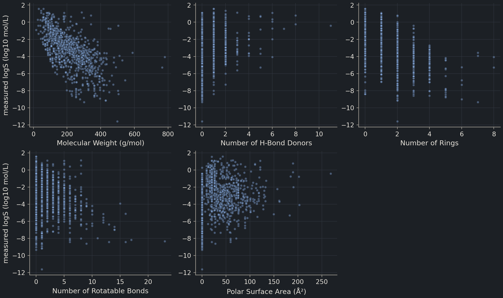
Draw a 2 × 3 grid of scatter plots of logS against each of the five descriptors, with alpha=0.4, labelled axes and the empty sixth panel removed with fig.delaxes(axes[1, 2]). Which panel shows the clearest trend, and which looks like a cloud with no structure?
SolutionShow solutionHide solution
fig, axes = plt.subplots(2, 3, figsize=(11, 6.5))for ax, col inzip(axes.flat, descriptors): ax.scatter(esol[col], esol[target], alpha=0.4, s=14) ax.set(xlabel=f"{col} ({units[col]})"if col in units else col)axes[0, 0].set(ylabel="measured logS (log10 mol/L)")axes[1, 0].set(ylabel="measured logS (log10 mol/L)")fig.delaxes(axes[1, 2])plt.show()
Molecular weight shows the clearest downward trend, and rings is a staircase of the same shape: each extra ring shifts the whole column of points down. The counts of donors and rotatable bonds are clouds; most compounds have 0 to 3 of each, and within those columns logS covers the full range. Polar surface area rises faintly. fig.delaxes removes the unused panel entirely, which is cleaner than leaving an empty set of axes in a figure that goes into a report.
Exercise★★★
Donors or no donors
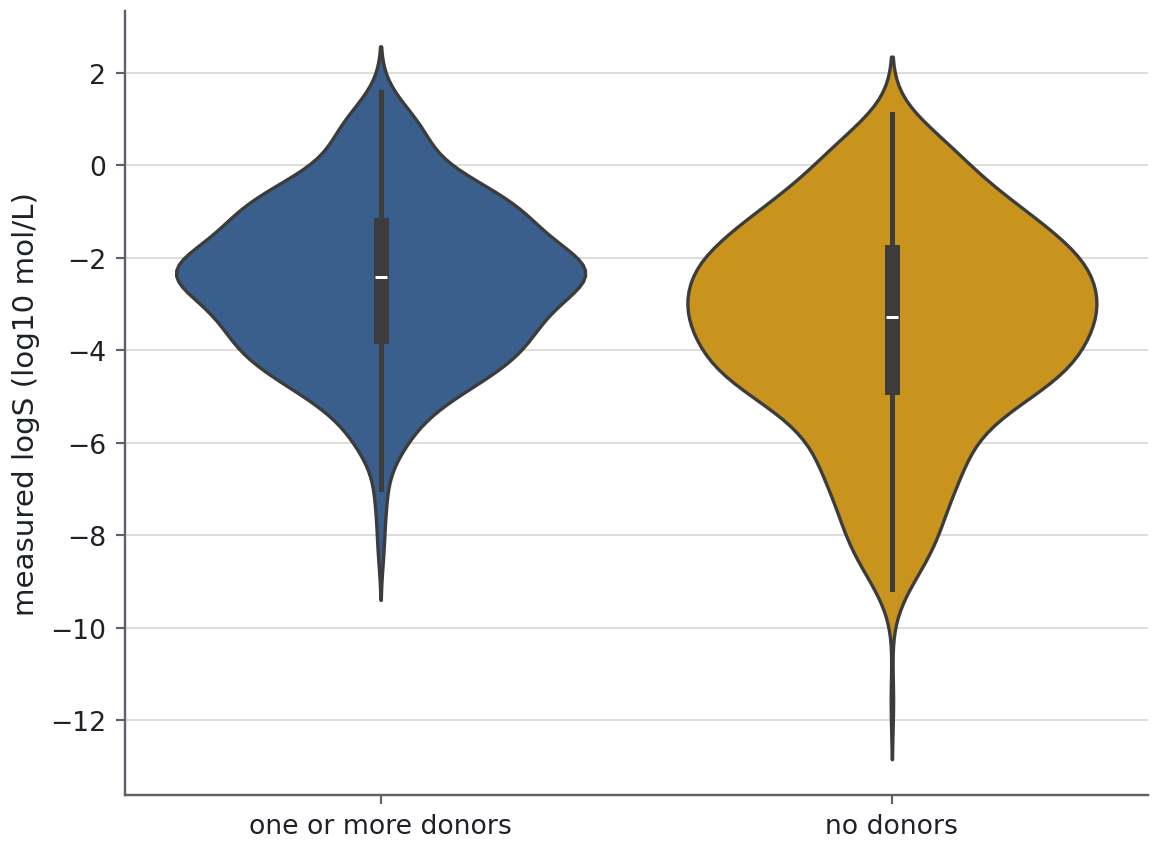
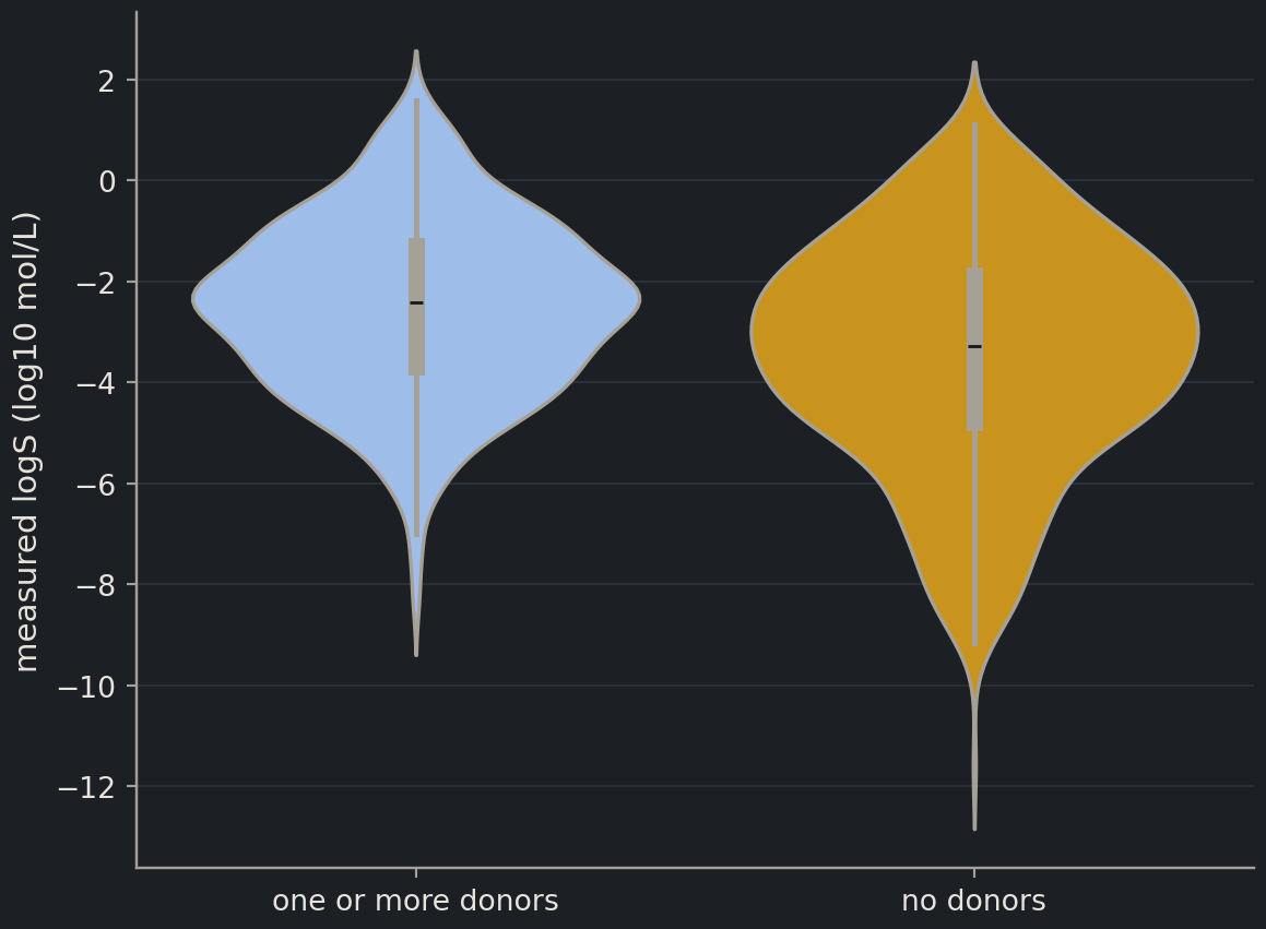
Hydrogen-bond donors should favour solubility. Make a new column that labels each compound as "no donors" or "one or more donors" (use np.where), draw a violin plot of logS for the two groups, and compute each group’s median. Is the effect large compared with the spread within each group? What does that tell you about using donor count as a predictor on its own?
SolutionShow solutionHide solution
import numpy as npesol = esol.assign( donor_group=np.where(esol["Number of H-Bond Donors"] >0, "one or more donors", "no donors"))esol.groupby("donor_group")[target].agg(["count", "median", "mean", "std"]).round(2)
Compounds with at least one donor are more soluble by about 0.85 log units at the median (−2.4 versus −3.3), a factor of about seven in solubility, so the effect is real and in the expected direction. But the standard deviation within each group is about 2 log units, more than twice the shift between them, and the violins overlap over nearly their whole length. Knowing only whether a molecule has a donor would tell you very little about its solubility; the descriptor is useful in combination with size and ring count, which is exactly what a multi-feature model is for. np.where(condition, a, b) is NumPy’s vectorised if/else, and assign returns a new frame rather than modifying esol in place.
Where this is going
Episode 2.1 takes the question you have just framed and defines what a model is; episode 2.2 fits a straight line through these five descriptors; and episode 2.3 measures how well it does, honestly, on compounds it has never seen. Everything you noticed today reappears there: the thin insoluble tail is where the model’s residuals will be largest, the redundancy between weight and rings is why regularisation helps in episode 2.4, and the smiles column, ignored until Chapter 5, is where the better features will come from.
Key points
Exploratory data analysis is the same short checklist every time: shape, types, missing values, the target’s distribution, each feature’s distribution, feature–target relationships, correlations, outliers, duplicates.
logS is log10 of solubility in mol/L: one unit is a factor of ten. Modelling the log turns a quantity spanning thirteen orders of magnitude into one a line can fit, and makes errors relative rather than absolute.
In ESOL, molecular weight (r ≈ −0.64) and ring count (r ≈ −0.51) are the descriptors most strongly related to solubility; hydrogen-bond donors and polar surface area help weakly.
The extremes make chemical sense: tiny polar molecules at the top, large chlorinated or polyaromatic hydrocarbons at the bottom. Outliers that make sense stay in.
ESOL contains no duplicated SMILES strings or compound names, but two different strings can describe one molecule; a chemistry toolkit (Chapter 5) is needed to be sure.
A SMILES string is a molecule written as text. Every descriptor in this file was computed from it, and so will yours be.