2.2 Linear regression from scratch, then scikit-learn
40 min of teaching20 min of exercisesbeginner
Questions this episode answers
How does a computer actually find the best straight line through data?
What are the normal equation and gradient descent, and when would I use each?
What do scikit-learn’s fit, predict and score do, and what is in coef_ and intercept_?
Can I read a regression coefficient as the effect of that feature?
What you will be able to do
Write the linear model \(\hat{y} = \theta_0 + \theta_1 x\) and its mean-squared-error loss as NumPy code.
Solve for the least-squares parameters with the normal equation using np.linalg.solve.
Implement gradient descent with an explicit loop, plot the loss curve and choose a learning rate that converges.
Fit the same model with LinearRegression and use the fit / predict / score estimator API.
Fit a linear model on five descriptors and interpret its coefficients with the right caveats about correlation and units.
In episode 2.1 you scored two guessed lines through the solubility data by their mean squared error and found that the sloping one was better. Guessing is not a method. This episode lets the computer find the best line, three times over: once with an exact formula, once by walking downhill, and once by calling scikit-learn. The three agree to a dozen decimal places, and seeing why they agree is what makes the scikit-learn call, which you will type a thousand times, something you understand rather than something you copy.
Everything here is fitted to all 1,128 molecules and judged on the same molecules. That is deliberate and temporary: the goal of this episode is to understand the fitting machinery, and episode 2.3 adds the held-out data you need before any number here can be called a result.
One descriptor, one line
Load the ESOL data as in episode 1.5 and take two columns: molecular weight as the single featurefeatureAn input variable describing a sample; one column of the X matrix.\(x\), and logSlogSThe base-10 logarithm of aqueous solubility in mol/L; the ESOL target. as the labellabelThe quantity you want to predict for each sample; the vector y.\(y\). For the from-scratch part we work with NumPy arrays rather than pandas columns, so that the maths and the code line up exactly.
from pathlib import Pathimport numpy as npimport pandas as pdESOL_URL ="https://deepchemdata.s3-us-west-1.amazonaws.com/datasets/delaney-processed.csv"path = Path("data/esol.csv")esol = pd.read_csv(path if path.exists() else ESOL_URL)x = esol["Molecular Weight"].to_numpy()y = esol["measured log solubility in mols per litre"].to_numpy()n =len(x)print(f"{n} molecules; x in g/mol from {x.min():.1f} to {x.max():.1f}; y in log10 mol/L")
1128 molecules; x in g/mol from 16.0 to 780.9; y in log10 mol/L
The modelmodelA function f(x; θ) with adjustable parameters θ that maps features to a prediction. is a straight line with two parametersparameterA number inside a model that training adjusts, such as a regression coefficient., an intercept \(\theta_0\) and a slope \(\theta_1\):
\[
\hat{y} = \theta_0 + \theta_1 x .
\]
The loss functionloss functionA number that measures how wrong a model’s predictions are; training means making it small. is the MSEmean squared error (MSE)The average of the squared prediction errors; the usual loss for regression., the average squared gap between measured and predicted values,
and fitting means finding the \((\theta_0, \theta_1)\) that makes \(L\) smallest. In code:
def predict(theta, x):"""Predictions of the line theta[0] + theta[1] * x."""return theta[0] + theta[1] * xdef mse(theta, x, y):"""Mean squared error of the line with parameters theta on (x, y)."""return np.mean((y - predict(theta, x)) **2)print(f"loss of the guess (-0.4, -0.013): {mse(np.array([-0.4, -0.013]), x, y):.4f}")
loss of the guess (-0.4, -0.013): 2.5915
The guess from episode 2.1 scores 2.59. Two methods will now find the parameters that score the minimum.
The exact answer: the normal equation
Stack the two parameters into a vector \(\theta = (\theta_0, \theta_1)\) and put the data into a design matrix\(X\) with one row per molecule and two columns: a column of ones (which multiplies the intercept) and the column of molecular weights. Then all \(n\) predictions at once are a single matrix–vector product, \(\hat{y} = X\theta\).
Why the column of ones? Row \(i\) of \(X\theta\) is \(1\cdot\theta_0 + x_i\theta_1\), exactly the line. The trick lets the intercept be treated like any other parameter, and it is why “a linear model” and “a matrix product” are the same thing for the rest of this course.
The MSE is a bowl-shaped function of \(\theta\) (a quadratic that opens upwards), so it has exactly one minimum, at the point where every partial derivative is zero. Setting the derivatives to zero and rearranging (the deep dive below does it) gives the normal equationnormal equationThe linear system XᵀXθ = Xᵀy whose solutions minimise the squared error of a linear model.:
\[
(X^\top X)\,\theta = X^\top y .
\]
This is a system of two linear equations in two unknowns, and NumPy solves such systems in one call.
theta_ne = np.linalg.solve(X.T @ X, X.T @ y)print(f"intercept {theta_ne[0]:.5f} slope {theta_ne[1]:.5f} logS per g/mol")print(f"loss at the minimum: {mse(theta_ne, x, y):.4f}")
intercept -0.38597   slope -0.01306 logS per g/mol
loss at the minimum: 2.5915
The slope says that each extra 100 g/mol of molecular weight costs about 1.3 log units of solubility, a factor of twenty, if nothing else changes. The loss, 2.59, is barely below the guess from episode 2.1 (which was, in fact, a rounded version of this answer).
Tip
solve, not inv
You will see \(\theta = (X^\top X)^{-1} X^\top y\) in textbooks, and the literal translation np.linalg.inv(X.T @ X) @ X.T @ y is tempting. Do not. Computing an explicit inverse and then multiplying costs more and loses precision; np.linalg.solve factorises the matrix and solves the system directly, which is both faster and more accurate, especially when the columns of \(X\) are nearly collinear (as they will be with real descriptors). The inverse is a thing you write; solve is the thing you compute.
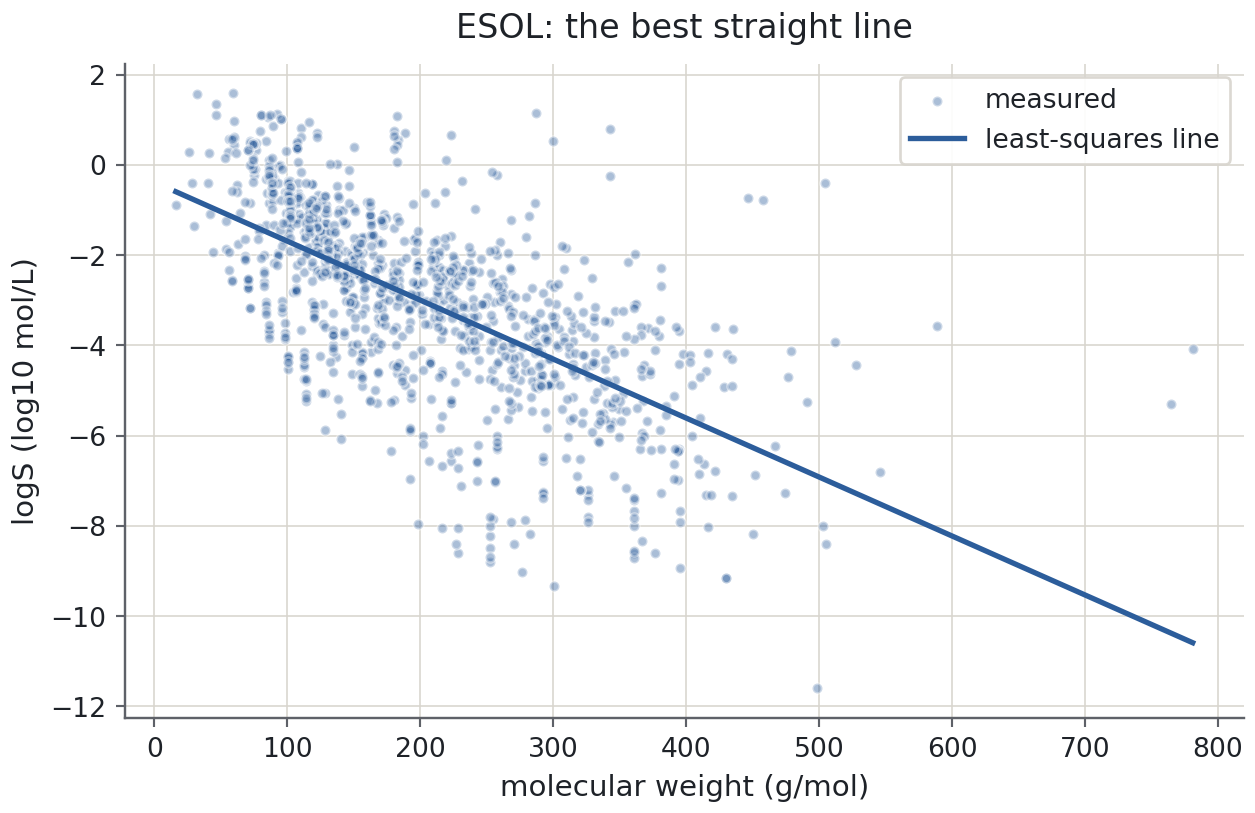
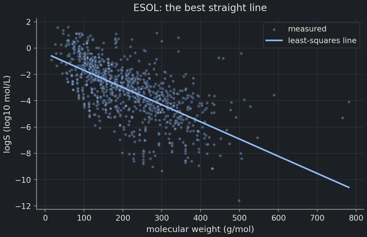
import matplotlib.pyplot as pltgrid = np.linspace(x.min(), x.max(), 100)fig, ax = plt.subplots(figsize=(6.5, 4.2))ax.scatter(x, y, alpha=0.4, s=14, label="measured")ax.plot(grid, predict(theta_ne, grid), linewidth=2, label="least-squares line")ax.set(xlabel="molecular weight (g/mol)", ylabel="logS (log10 mol/L)", title="ESOL: the best straight line")ax.legend()plt.show()
The line captures the trend and misses a great deal: at any molecular weight the measured values spread over four or five log units. Molecular weight is one of several things that matter, which is why the episode ends with five descriptors.
Deep diveDeriving the MSE gradientShow the mathsHide the maths
Write the loss in matrix form, with \(r = y - X\theta\) the vector of residuals:
Differentiating with respect to the vector \(\theta\) (each component \(\partial L/\partial\theta_j\) collected into one vector) uses the chain rule: the derivative of \(r^\top r\) with respect to \(r\) is \(2r\), and the derivative of \(r\) with respect to \(\theta\) is \(-X\). Hence
\[
\nabla_\theta L = \frac{1}{n}\cdot 2\,(-X)^\top r = -\frac{2}{n}\,X^\top (y - X\theta).
\]
At the minimum the gradientgradientThe vector of partial derivatives; it points in the direction of steepest increase. vanishes:
which is the normal equation. The solution is unique whenever \(X^\top X\) is invertible, that is, whenever no column of \(X\) is an exact linear combination of the others. The same gradient, with the sign flipped, is the step direction of gradient descent below.
Maths corner
Least squares is a projection. The vector of predictions \(X\theta\) ranges over the column space of \(X\) (a plane through the origin in \(\mathbb{R}^n\) when \(X\) has two columns), and minimising \(\|y - X\theta\|^2\) means choosing the point of that plane closest to \(y\), its orthogonal projection. The residual \(y - X\hat\theta\) is therefore perpendicular to every column of \(X\): \(X^\top(y - X\hat\theta) = 0\), which is the normal equation again, read geometrically. The maths refresher covers the vector and projection facts used here.
Chemist's corner
You have fitted this model every time you made a calibration curve. Beer–Lambert says absorbance \(A = \varepsilon\,l\,c\): a straight line through standards of known concentration \(c\), slope \(\varepsilon l\), intercept ideally zero. Fitting the standards by least squares is the normal equation with \(x = c\) and \(y = A\); the “unknown” is then read off by inverting the line. Everything that makes a calibration curve trustworthy (standards that span the working range, replicates, checking for curvature at high absorbance) has a counterpart in this chapter.
The iterative answer: gradient descent
The normal equation works because the MSE of a linear model is a bowl with a formula for its bottom. Most models in this course, from logistic regression onwards, have no such formula. What they have is a gradient, and that is enough.
Picture the loss as a landscape over the two parameters, with the minimum at the bottom of a valley, and yourself standing somewhere on the slope in fog. You cannot see the bottom, but you can feel which way the ground tilts under your feet. The gradientgradientThe vector of partial derivatives; it points in the direction of steepest increase. is that tilt, the direction of steepest ascent. Take a step the other way, feel the tilt again, repeat. That is gradient descentgradient descentImproving parameters step by step by moving against the gradient of the loss.:
The number \(\eta\) (eta) is the learning ratelearning rateThe step size of gradient descent; too large diverges, too small crawls.: how far you step each time. Too small and you crawl; too large and you overshoot the valley and climb the far side.
One preparation first. The two parameters live on very different scales: \(\theta_0\) is in log units and \(\theta_1\) in log units per g/mol, with \(x\) running from 16 to 781. The loss landscape is then a long, narrow trench rather than a round bowl, and a step size that is safe along the trench is far too big across it. The cure is to standardise\(x\): subtract its mean and divide by its standard deviation, so that the feature has mean 0 and spread 1. The exercise on unstandardised data shows what happens without this.
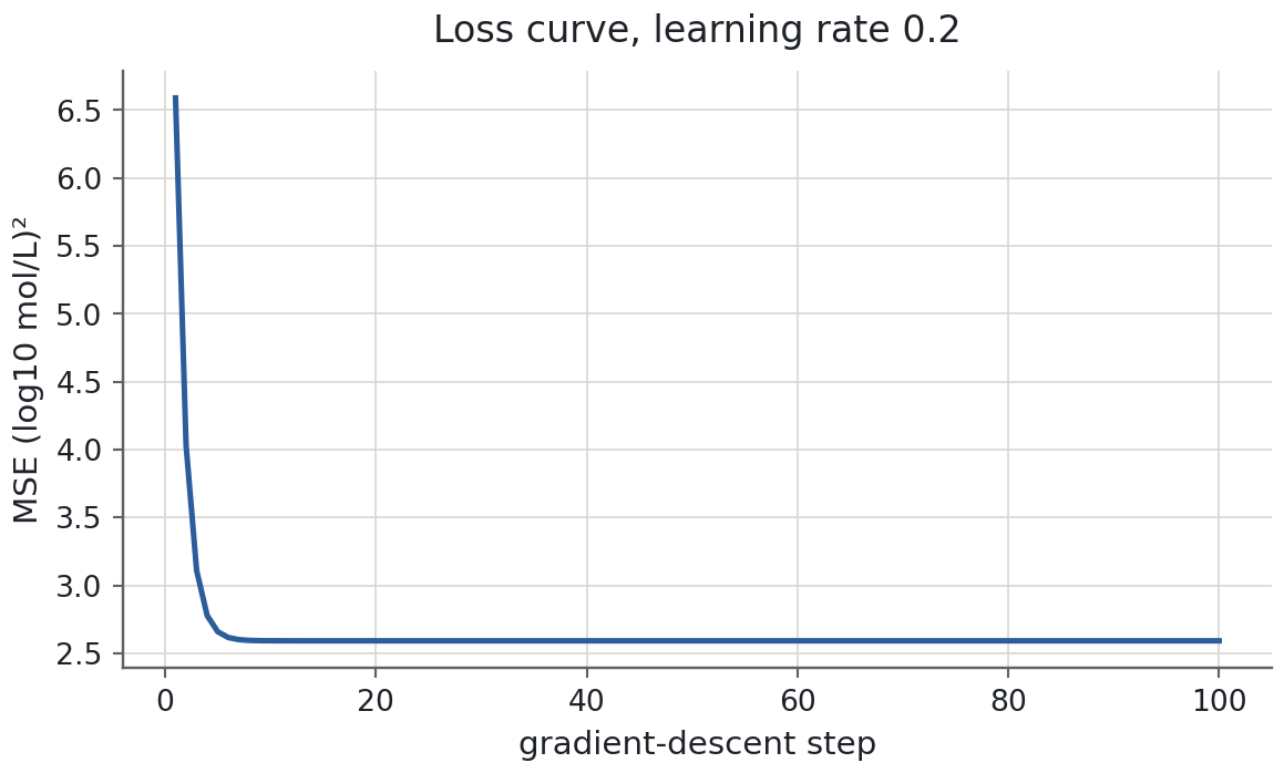
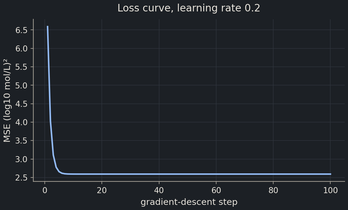
The loss falls steeply for the first ten or so steps and then flattens at 2.59, the same minimum the normal equation found. The parameters look different (−3.05 and −1.34) only because they describe the line in standardised units; converting them back recovers the earlier slope and intercept exactly.
gradient descent, original units: intercept -0.38597  slope -0.01306
normal equation:                  intercept -0.38597  slope -0.01306
Note
When would you ever use this?
For a linear model with a few thousand rows, never; the normal equation is exact and instant. Gradient descent earns its place when there is no closed form (almost every model after this one), when the data are too large to hold \(X^\top X\) in memory, or when the data arrive in a stream. Chapter 4 trains neural networks with precisely the loop above, with a longer gradient line.
Choosing the learning rate
Predict before you run
The loop above used \(\eta = 0.2\). Suppose you make the learning rate ten times larger, \(\eta = 2\). Will the loss reach the minimum faster, reach it more slowly, or never reach it? Sketch the loss curve you expect before you run the next cell.
theta = np.zeros(2)for step inrange(5): gradient =-2/ n * Z.T @ (y - Z @ theta) theta = theta -2.0* gradientprint(f"step {step +1}: loss = {mse(theta, z, y):,.0f}")
step 1: loss = 103
step 2: loss = 902
step 3: loss = 8,097
step 4: loss = 72,848
step 5: loss = 655,612
Every step makes the loss roughly nine times worse. With \(\eta = 2\) each step overshoots the valley floor and lands higher up the opposite wall than where it started; the parameters alternate in sign and grow without bound. A few more steps and the numbers overflow. With \(\eta = 0.2\) the same loop converged in thirty steps; with \(\eta = 0.002\) it would still be creeping after a thousand. The loss curve is how you tell the three cases apart: diverging (up), crawling (down but still sloping at the end) or converged (flat).
Common mistake
A flat loss curve is not always good news
A loss curve that is flat from the first step is as suspicious as one that explodes. It usually means the learning rate is so small that nothing is moving, or that a bug has made the gradient zero. Print the first few losses and the first few parameter values; if neither changes, the loop is not doing what you think.
The same fit with scikit-learn
You will never write the normal equation by hand in a project. scikit-learn’s LinearRegression does it (with a more careful numerical method) and wraps the result in an interface you will use for every model in this course. Fit it on the single feature and compare with the hand-made answer. The feature table must be two-dimensional, one column per feature, so we pass a one-column DataFrame.
Identical to ten decimals: there is nothing inside LinearRegression that you have not just done yourself. What scikit-learn adds is a contract. Every model in the library is an estimatorestimatorAny scikit-learn object with fit and predict (or transform) methods., an object with the same four pieces:
fit(X, y) learns the parameters from the data and stores them on the object;
predict(X) applies the learned function to new rows of X;
score(X, y) returns a default quality measure (for regressors it is \(R^2\); what that is and when it lies is for episode 2.3);
learned quantities are attributes with a trailing underscore, here coef_ and intercept_, which exist only after fit.
new_molecules = pd.DataFrame({"Molecular Weight": [100.0, 300.0, 500.0]})print("predicted logS:", linreg.predict(new_molecules).round(2))print(f"R² on the training data: {linreg.score(esol[['Molecular Weight']], y):.3f}")
predicted logS: [-1.69 -4.31 -6.92]
R² on the training data: 0.410
The predictions are what the line gives at 100, 300 and 500 g/mol, and the training \(R^2\) of 0.41 says that molecular weight alone accounts for about 40% of the variation in logS. Remember the caveat from the top of the episode: this is a score on the data the line was fitted to, and it will flatter every model you ever build.
For programmers
The estimator API is a protocol (an interface, a duck type): anything with fit and predict is a regressor as far as the rest of scikit-learn is concerned, whether it is a line, a forest or a neural network. That is why the evaluation code in 2.3, the cross-validation in 2.4 and the pipelines in 2.6 take a model as an argument and never ask what kind it is. fit returns self, so LinearRegression().fit(X, y) chains, and the trailing-underscore convention lets you tell learned state (coef_) from configuration set in the constructor (fit_intercept) at a glance.
Common mistake
X must be two-dimensional
linreg.fit(esol["Molecular Weight"], y) with single brackets raises an error, because a pandas Series is one-dimensional and scikit-learn insists on the X / y conventionX / y conventionFeatures in a 2-D array X of shape (n_samples, n_features); targets in a 1-D array y.: X has shape (n_samples, n_features) even when there is one feature. Use double brackets, esol[["Molecular Weight"]], or x.reshape(-1, 1) for a NumPy array. The error message says exactly this, but it is the first scikit-learn error almost everyone meets.
Five descriptors at once
Nothing in the normal equation, the gradient or the estimator cared that \(X\) had two columns. Give it six (a column of ones plus five molecular descriptorsmolecular descriptorA number computed from a molecule’s structure, such as molecular weight or polar surface area.) and the same equation fits a model with six parameters:
With LinearRegression the only change is the width of X. We fit on all 1,128 molecules; there is no train/test split here, on purpose, because evaluation is the subject of the next episode and this one is about the fit.
features = ["Molecular Weight","Number of H-Bond Donors","Number of Rings","Number of Rotatable Bonds","Polar Surface Area",]X5 = esol[features]model5 = LinearRegression().fit(X5, y)coefs = pd.DataFrame({"coefficient": model5.coef_}, index=pd.Index(features, name="feature"))print(f"intercept: {model5.intercept_:.3f} training R²: {model5.score(X5, y):.3f}")coefs.round(4)
intercept: -0.580 training R²: 0.683
index
coefficient
feature
index
Molecular Weight
-0.0131
Number of H-Bond Donors
0.0731
Number of Rings
-0.4724
Number of Rotatable Bonds
-0.1509
Polar Surface Area
0.0323
Each coefficientcoefficientThe weight a linear model gives to one feature; its sign and size are only interpretable with care. is the change in predicted logS for a one-unit increase in that feature while the other four are held fixed. Read down the table: heavier molecules, more rings and more rotatable bonds all predict lower solubility; more hydrogen-bond donors and more polar surface area predict higher. All five signs agree with chemical intuition about what dissolves in water, and together they lift the training \(R^2\) from 0.41 to 0.68.
Chemist's corner
Suppose the coefficient on polar surface area had come out negative. Taken literally that would say that making a molecule more polar, with everything else fixed, makes it less water-soluble, which contradicts everything you know about hydrogen bonding and solvation. The right response is not to invent a mechanism but to suspect the model: polar surface area and hydrogen-bond donors are strongly correlated, and when two features carry nearly the same information the fit can hand all the credit to one and a compensating, meaningless, sign to the other. The next section shows this happening with the ring count.
Reading coefficients carefully
A coefficient is a property of the model, not of the molecule, and two things about the model change it without changing the chemistry.
Correlated features. The five descriptors are not independent. The correlation coefficientcorrelation coefficientA number between −1 and 1 measuring how linearly two variables move together. matrix shows that ring count rises with molecular weight (\(r \approx 0.65\)) and that polar surface area rises with the number of hydrogen-bond donors (\(r \approx 0.76\)).
X5.corr().round(2)
index
Molecular Weight
Number of H-Bond Donors
Number of Rings
Number of Rotatable Bonds
Polar Surface Area
Molecular Weight
1.00
0.25
0.65
0.40
0.48
Number of H-Bond Donors
0.25
1.00
0.21
0.08
0.76
Number of Rings
0.65
0.21
1.00
-0.14
0.31
Number of Rotatable Bonds
0.40
0.08
-0.14
1.00
0.29
Polar Surface Area
0.48
0.76
0.31
0.29
1.00
When two features move together, the model has a choice about how to share the effect between them, and the choice depends on which other features are present. Remove the ring count and refit.
without_rings = [f for f in features if f !="Number of Rings"]model4 = LinearRegression().fit(esol[without_rings], y)comparison = coefs.rename(columns={"coefficient": "with rings"})comparison["without rings"] = pd.Series(model4.coef_, index=without_rings)comparison.round(4)
index
with rings
without rings
feature
index
index
Molecular Weight
-0.0131
-0.0180
Number of H-Bond Donors
0.0731
0.0783
Number of Rings
-0.4724
NaN
Number of Rotatable Bonds
-0.1509
-0.0383
Polar Surface Area
0.0323
0.0311
The coefficient on rotatable bonds shrinks to a quarter of its size and the one on molecular weight grows by a third, although neither feature changed. With ring count gone, molecular weight takes over the job of describing large, ring-rich molecules, and rotatable bonds no longer need to compensate. Neither set of coefficients is “the effect of molecular weight on solubility”; each is the best division of labour among the features it was given.
Units and scale. A coefficient is per unit of the feature, so it changes with the units you chose. Express molecular weight in kg/mol instead of g/mol and the coefficient becomes a thousand times larger while the model, its predictions and its \(R^2\) stay identical.
A bigger coefficient is not a more important feature
In the table above the ring coefficient (−0.47) is thirty times the molecular-weight coefficient (−0.013). That says nothing about importance: one ring is one unit, while one g/mol is a tiny step on a feature that spans 760 units. To compare features you must put them on the same scale first, which is one of the reasons episode 2.6 standardises features inside a pipeline. Until then, read signs with care and magnitudes not at all.
Exercises
Exercise★☆☆
Linear in what?
“Linear regression” means linear in the parameters, not in the feature. Which of these models can the normal equation fit as they stand, and which cannot? For the ones it can, say what the columns of the design matrix would be.
\(\hat{y} = \theta_0 + \theta_1 x^2\)
\(\hat{y} = \theta_0\,e^{\theta_1 x}\)
\(\hat{y} = \theta_0 + \theta_1 \log x + \theta_2 \sqrt{x}\)
\(\hat{y} = \theta_0 + \theta_1 x + \theta_2 x^2\)
SolutionShow solutionHide solution
Yes. Columns: a column of ones and a column of \(x^2\). The feature is squared, but the prediction is still a weighted sum of known columns.
No.\(\theta_1\) sits inside the exponential, so the prediction is not a weighted sum of fixed columns. (Taking logs of both sides gives \(\log\hat{y} = \log\theta_0 + \theta_1 x\), which is linear in new parameters, but that fits a different loss, on \(\log y\).)
Yes. Columns: ones, \(\log x\), \(\sqrt{x}\). Any fixed transformation of the features is allowed.
Yes. Columns: ones, \(x\), \(x^2\). This is the polynomial fit of episode 2.1 written as a linear model, which is why PolynomialFeatures followed by LinearRegression is how scikit-learn fits polynomials; episode 2.4 uses exactly that.
The rule: if you can write \(\hat{y} = X\theta\) for some matrix \(X\) built from the features before you know \(\theta\), the normal equation applies.
Exercise★☆☆
Normal equation for five features
Build the design matrix for the five descriptors (a column of ones followed by the five columns of X5), solve the normal equation with np.linalg.solve, and compare the six numbers with model5.intercept_ and model5.coef_.
largest difference from sklearn: 6.5503158452884236e-15
intercept                   -0.5796
Molecular Weight            -0.0131
Number of H-Bond Donors      0.0731
Number of Rings             -0.4724
Number of Rotatable Bonds   -0.1509
Polar Surface Area           0.0323
dtype: float64
The two agree to about \(10^{-12}\) or better, which is the precision of floating-point arithmetic on a problem of this size, not a coincidence: both minimise the same loss, which has one minimum. The only thing LinearRegression does differently is to use a numerically more careful method (a least-squares solver rather than forming \(X^\top X\)), which matters when the columns are nearly collinear.
Exercise★★☆
Gradient descent without standardising
Run the gradient-descent loop on the unstandardised design matrix X (ones and raw molecular weight) with the learning rate that worked before, \(\eta = 0.2\), for five steps and print the losses. Then find a learning rate for which the loss decreases, run 200 steps, and compare the parameters with the normal equation. Explain what you see.
eta = 0.2, step 1: loss = 4.82e+09
eta = 0.2, step 2: loss = 2.09e+18
eta = 0.2, step 3: loss = 9.11e+26
eta = 0.2, step 4: loss = 3.96e+35
eta = 0.2, step 5: loss = 1.72e+44
eta = 1e-5, after 200 steps: intercept -0.0004  slope -0.01457
normal equation:             intercept -0.3860  slope -0.01306
With \(\eta = 0.2\) the loss explodes within five steps, far faster than the standardised case with \(\eta = 2\). Raw molecular weight is in the hundreds, so the slope component of the gradient is tens of thousands of times larger than the intercept component, and a step that was gentle for standardised \(z\) is enormous for \(x\).
With \(\eta = 10^{-5}\) the loss decreases and the slope is essentially right after 200 steps, but the intercept has barely moved from zero: the step size that is safe for the steep slope direction is far too timid for the shallow intercept direction. In the long, narrow trench of the unstandardised loss landscape no single learning rate suits both parameters. Standardising makes the trench round, so that one \(\eta\) serves every direction, which is why every gradient-based method in this course, including neural networks, is preceded by feature scaling.
Exercise★★★
A squared term
Add a sixth feature, molecular weight squared, to X5 and refit LinearRegression. Does the training \(R^2\) improve? Print the coefficients on molecular weight and its square. Then say, in two sentences, why this improvement is not evidence that the squared term helps.
SolutionShow solutionHide solution
X6 = X5.assign(**{"MW squared": X5["Molecular Weight"] **2})model6 = LinearRegression().fit(X6, y)print(f"training R²: five features {model5.score(X5, y):.4f} with MW² {model6.score(X6, y):.4f}")print(f"coefficient on MW: {model6.coef_[0]:.5f} on MW²: {model6.coef_[-1]:.2e}")
training R²: five features 0.6831   with MW²  0.7066
coefficient on MW: -0.02278   on MW²: 1.97e-05
The training \(R^2\) rises from 0.683 to about 0.707, and the coefficients say the fitted curve in molecular weight bends slightly upwards (negative linear term, small positive quadratic term), so the solubility penalty per g/mol eases off for the heaviest molecules.
Why this is not evidence: adding any column to \(X\) can never increase the minimum of the training loss, because the model with that coefficient set to zero is still available, so the training \(R^2\) rises for every added feature, informative or not. Episode 2.1’s degree-15 polynomial is the extreme case. Whether the squared term helps with new molecules is a question only held-out data can answer, and episode 2.3 is where you get to ask it. Note also that MW and MW² are highly correlated, so the two coefficients should be read together, as a curve, not separately.
Where this is going
The line you fitted today is the model that Chapter 6 fits with hundreds of descriptors and fingerprint bits instead of five, where the coefficient problems of the last section stop being a curiosity and become the central difficulty, and where ridge and lasso regression (episode 2.4) are the standard response. The gradient-descent loop is the model that Chapter 4 fits: a neural network is \(f(x;\theta)\) with millions of parameters, the gradient comes from automatic differentiation rather than a one-line formula, and the step rule \(\theta \leftarrow \theta - \eta\nabla L\) is unchanged, learning rate and all. Before either, episode 2.3 answers the question this episode has carefully avoided: is the model any good?
Key points
A linear model predicts ; fitting means choosing to minimise the mean squared error on the training data.
The normal equation gives the exact least-squares solution in one line: solve with np.linalg.solve, never with an explicit inverse.
Gradient descent reaches the same answer step by step: compute the gradient, move against it, repeat. The learning rate decides whether it converges, crawls or explodes.
Standardise features before gradient descent. The normal equation does not care about scale; gradient descent does.
scikit-learn wraps all of this in the estimator API: fit, predict, score, coef_, intercept_. Every model in this course uses the same names.
Coefficients are not effects. They depend on the units of the feature and on which other, correlated features are in the model.
Everything in this episode is fitted and scored on the same data. Whether the model is any good is the question of episode 2.3.