Why can’t I judge a model on the data it was trained on?
What is a baseline, and why must every model beat one?
Which numbers (MAE, RMSE, R²) tell me how good a regression model is, and what do they hide?
What you will be able to do
Split data into training and test sets reproducibly with train_test_split and random_state.
Build a baseline with DummyRegressor and compare a real model against it.
Compute and interpret MAE, RMSE and R² on held-out data.
Read a parity plot and a residual plot to find where a model fails.
In episode 2.2 you fitted a linear model that predicts the aqueous solubility of small molecules from a handful of molecular descriptorsmolecular descriptorA number computed from a molecule’s structure, such as molecular weight or polar surface area.. The fit looked reasonable. But looked reasonable is not a scientific statement, and the number you printed at the end, the \(R^2\) on the data you fitted, is not evidence of anything. This episode is about replacing that feeling with a procedure you can defend.
The procedure has three parts, and you will use all three in every later chapter of this course, whether the model predicts solubility, protein function or the quality of a docked pose:
Hold data back before you fit anything, and measure the model only on that held-back data.
Beat a baselinebaselineA deliberately simple model (such as predicting the mean) that any real model must beat.. A trivial model sets the bar; a real model has to clear it.
Use the right numbers and the right pictures. One summary metric hides as much as it shows.
Why training performance is not evidence
Imagine a student who memorises the answers to last year’s exam. On that exam they score 100%. On this year’s exam they do no better than anyone else. Their score on the memorised paper told you nothing about their understanding, because the questions were the same ones they had seen.
A model is in exactly that position when you evaluate it on the data it was trained on. Training adjusts the parameters \(\theta\) to make the loss functionloss functionA number that measures how wrong a model’s predictions are; training means making it small. small on those particular examples. A flexible enough model can drive the training error to zero by memorising noise, molecule by molecule, without learning anything that transfers. The goal of machine learning is generalisationgeneralisationHow well a model performs on data it was not trained on., performance on examples the model has never seen, and the only way to measure generalisation is to keep some examples away from the model and test on them afterwards.
Biologist's corner
This is the same logic as a blinded experiment. If the person scoring the cells knows which wells got the drug, the readout is contaminated. The test settest setHeld-back data used once, at the end, to estimate performance on unseen examples. is your blinded replicate: the model never sees it, so it cannot cheat.
The simplest version of this idea is the train/test splittrain/test splitDividing the data into a part the model learns from and a part kept back to measure it honestly.: shuffle the rows, use most of them (typically 70–80%) to fit the model, and keep the rest as a test settest setHeld-back data used once, at the end, to estimate performance on unseen examples. that you touch exactly once, at the end.
Setting up: the solubility data again
We continue with the ESOL dataset from episode 1.5. The target is logSlogSThe base-10 logarithm of aqueous solubility in mol/L; the ESOL target., the base-10 logarithm of solubility in mol/L, and the features are five descriptors that come with the file. (In Chapter 5 you will compute descriptors like these yourself with RDKit.)
from pathlib import Pathimport numpy as npimport pandas as pdESOL_URL ="https://deepchemdata.s3-us-west-1.amazonaws.com/datasets/delaney-processed.csv"path = Path("data/esol.csv")esol = pd.read_csv(path if path.exists() else ESOL_URL)features = ["Molecular Weight","Number of H-Bond Donors","Number of Rings","Number of Rotatable Bonds","Polar Surface Area",]X = esol[features]y = esol["measured log solubility in mols per litre"]X.shape, y.shape
((1128, 5), (1128,))
As always, X has one row per sample (molecule) and one column per featurefeatureAn input variable describing a sample; one column of the X matrix., and y has one labellabelThe quantity you want to predict for each sample; the vector y. per row.
Splitting reproducibly
scikit-learn’s train_test_split shuffles the rows and divides them. Two arguments matter:
test_size=0.2 keeps 20% of the molecules back.
random_state=42 fixes the shuffle, so that you, your colleague and this website all get the same split. Any fixed integer works; 42 is a convention, not magic.
from sklearn.model_selection import train_test_splitX_train, X_test, y_train, y_test = train_test_split( X, y, test_size=0.2, random_state=42)print(f"training molecules: {len(X_train)} test molecules: {len(X_test)}")
training molecules: 902 test molecules: 226
Common mistake
The order of the four outputs
train_test_split returns X_train, X_test, y_train, y_test in that order: both X parts first, then both y parts. Writing X_train, y_train, X_test, y_test = ... is a very common bug that produces no error message, because the shapes still look plausible, and then silently trains the model on the wrong data. Check with X_train.shape and y_train.shape: the first dimension must match.
Without random_state, every run of the notebook would give a different split, different metrics and an irreproducible result. From here on, every random operation in this course fixes a seed.
The baseline: a model that knows nothing
Before judging any model, ask: what score would I get by doing something trivially simple? For regression, the standard trivial model predicts the mean of the training targets for every molecule, whatever its features. scikit-learn ships it as DummyRegressor.
from sklearn.dummy import DummyRegressorbaseline = DummyRegressor(strategy="mean")baseline.fit(X_train, y_train)baseline.predict(X_test[:5])
Every prediction is the same number, the mean logS of the training set. This is the bar. A model that does not clearly beat it has not extracted any information from the features.
Note
There is a DummyClassifier too
For classification problems (Episode 2.5) the equivalent is DummyClassifier(strategy="most_frequent"), which always predicts the most common class. On a dataset where 90% of compounds are inactive, this baseline scores 90% accuracy while finding zero active compounds. Keep that in mind when someone reports “90% accuracy” without a baseline.
Three numbers for regression
Now fit the real model from episode 2.2, a LinearRegression on the five descriptors, and compute three metrics on the test set. Each metric compares the true values \(y_i\) with the predictions \(\hat{y}_i\) over the \(n\) test molecules.
Metric
Formula
Reads as
MAEmean absolute error (MAE)The average size of the prediction errors, in the units of the target.
\(\frac{1}{n}\sum_i |y_i - \hat{y}_i|\)
the typical error, in logS units
RMSEroot mean squared error (RMSE)The square root of the average squared error; it punishes large errors more than MAE does.
\(\sqrt{\frac{1}{n}\sum_i (y_i - \hat{y}_i)^2}\)
like MAE, but large errors count more
R²coefficient of determination (R²)The fraction of the variance in the target that the model explains; 1 is perfect, 0 matches the mean baseline.
fraction of the variance explained; 1 is perfect, 0 equals the mean baseline
from sklearn.linear_model import LinearRegressionfrom sklearn.metrics import mean_absolute_error, r2_score, root_mean_squared_errorlinreg = LinearRegression()linreg.fit(X_train, y_train)def report(model, X, y):"""Return MAE, RMSE and R² of `model` on the data (X, y).""" pred = model.predict(X)return {"MAE": mean_absolute_error(y, pred),"RMSE": root_mean_squared_error(y, pred),"R2": r2_score(y, pred), }results = pd.DataFrame( {"baseline (test)": report(baseline, X_test, y_test),"linear (test)": report(linreg, X_test, y_test), }).Tresults.round(3)
index
MAE
RMSE
R2
baseline (test)
1.732
2.174
-0.000
linear (test)
0.904
1.212
0.689
Read the table row by row:
The baseline’s \(R^2\) is about zero, as it must be: \(R^2\) is defined relative to predicting the mean. (It is slightly negative because the test mean differs a little from the training mean.)
The linear model’s errors are roughly half the baseline’s, and it explains about 70% of the variance in logS. It has clearly learned something.
MAE and RMSE differ: RMSE is larger because a few molecules are predicted badly, and squaring makes those few dominate.
Chemist's corner
What does an RMSE of about 1.2 logS units mean at the bench? logS is a base-10 logarithm, so an error of 1.2 is a factor of \(10^{1.2} \approx 16\) in solubility, and the MAE of about 0.9 is a factor of about 8. For deciding whether a compound is “soluble enough” that is often useful; for a precise formulation it is not. Delaney’s original ESOL model, which also used clogP, reported errors of roughly 0.75 log units on his data. The dataset includes his predictions, and the stretch exercise below compares them with ours on the same test molecules.
Deep diveWhy RMSE is at least as large as MAEShow the mathsHide the maths
For any set of errors \(e_i = y_i - \hat{y}_i\), the quadratic mean is never smaller than the arithmetic mean of the absolute values:
This follows from the Cauchy–Schwarz inequality (or from Jensen’s inequality applied to the convex function \(x \mapsto x^2\)). Equality holds only when all \(|e_i|\) are identical. So the gap between RMSE and MAE is itself informative: a large gap means the error distribution has a heavy tail, that is, a few very badly predicted samples.
The gap between training and test
Now the key experiment. Evaluate the same fitted model on the data it was trained on, and compare.
Predict before you run
Before you run the next cell: will the training RMSE be lower than, higher than, or the same as the test RMSE? By how much, roughly? Write your guess down.
For this model the gap is small: a straight line through five descriptors is too rigid to memorise 900 molecules, so it generalises about as well as it fits. That will not stay true in episode 2.4, where you will fit polynomial and nearest-neighbour models whose training error is tiny and whose test error is terrible. The habit to build now is that the training score is a diagnostic (a large gap means overfittingoverfittingWhen a model learns the noise in its training data and so performs worse on new data.), never the headline result.
Common mistake
‘Score’ is not always what you think
Every scikit-learn regressor has a .score(X, y) method, and for regressors it returns \(R^2\). Calling linreg.score(X_train, y_train) and reporting it as “the model’s accuracy” is a double mistake: it is \(R^2\) rather than accuracy, and it is measured on the training set. Be explicit: compute the metric you mean, on the data you mean.
Pictures: parity plots and residuals
Metrics summarise. Plots explain. The two standard pictures for a regression model are:
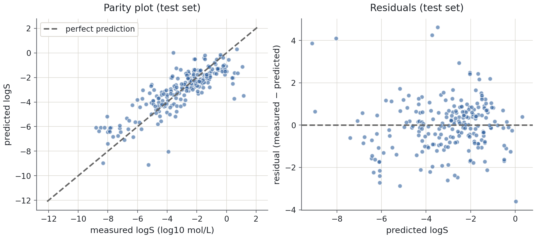
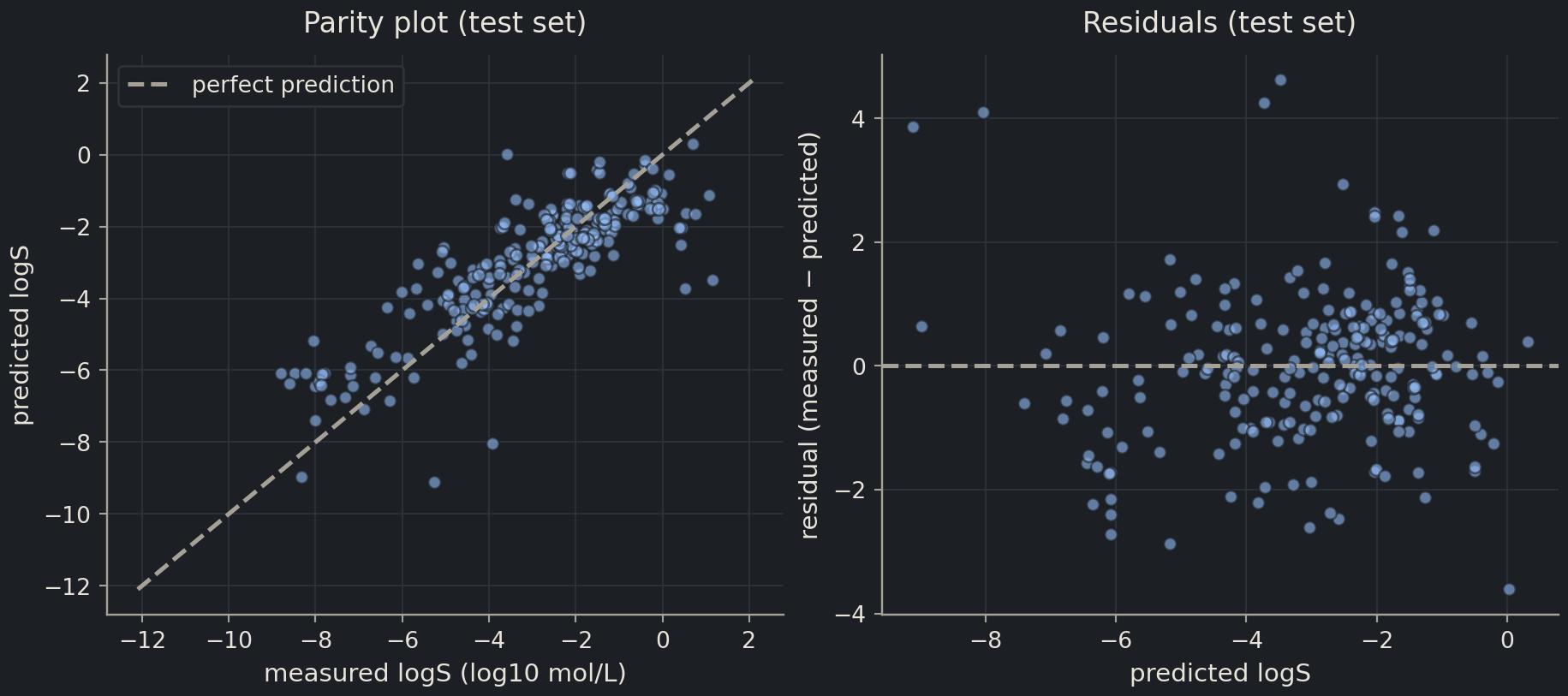
a parity plotparity plotA scatter plot of predicted against true values; perfect predictions lie on the diagonal.: predicted against true values, with the diagonal \(y = x\) marking perfect predictions;
a residualresidualThe difference between a true value and the model’s prediction for it. plot: the residual \(y_i - \hat{y}_i\) against the prediction, which should look like structureless noise around zero if the model has captured the signal.
At the insoluble end (measured logS below about −6) the model usually predicts values that are too high. These points sit above the diagonal because predicted logS is on the vertical axis; their measured-minus-predicted residuals are negative.
Several molecules have large individual errors, more than two log units in either direction, even though the average residual is near zero. The plot alone does not establish their cause: missing descriptors, a model that is too rigid, and unusual measurements are all possibilities to investigate.
The residuals also tell you which molecules are wrong. Looking at the worst cases is often the most valuable minute in a modelling project.
Scan the SMILES of the worst-predicted compounds. The biggest misses are typically very large, rigid, poorly soluble molecules whose logS is far below what their molecular weight alone suggests. Five whole-molecule descriptors carry no information about where the atoms are; the fingerprints and graph representations of Part II exist precisely to fix that.
How much does the split matter?
One split gives one number. If you had chosen random_state=7, which molecules landed in the test set would change, and so would the RMSE. Run the experiment ten times to see the spread.
rmses = []for seed inrange(10): Xtr, Xte, ytr, yte = train_test_split(X, y, test_size=0.2, random_state=seed) model = LinearRegression().fit(Xtr, ytr) rmses.append(root_mean_squared_error(yte, model.predict(Xte)))print(f"test RMSE over 10 splits: mean {np.mean(rmses):.3f}, "f"min {np.min(rmses):.3f}, max {np.max(rmses):.3f}")
test RMSE over 10 splits: mean 1.174, min 1.119, max 1.231
The spread is a few hundredths of a log unit for this dataset, so one split is adequate here. On small datasets (a few dozen measurements is common in chemistry and biology) the spread can be as large as the effect you are trying to detect, which is why episode 2.4 introduces cross-validationcross-validationRepeatedly splitting the data into folds so that every sample is tested on exactly once.: it repeats the split systematically so that every sample is tested once.
Discussion
A colleague reports “our model achieves R² = 0.93” for predicting a binding affinity from 80 measured compounds. List three questions you would ask before believing that number tells you anything about the next 80 compounds.
Exercises
Exercise★☆☆
Metrics by hand
A model predicts logS values of −2.0, −3.5 and −5.0 for three molecules whose measured values are −2.5, −3.0 and −6.0. Without code, compute the MAE and the RMSE. Which is larger, and why?
RMSE is larger because squaring gives the biggest error (1.0) more weight than the two smaller ones. The gap is small here because the errors are similar in size; a single error of 3.0 would push RMSE far above MAE.
Exercise★☆☆
Debug this
A labmate’s code runs without errors but their model “works perfectly”. Find two bugs.
Unpacking order.train_test_split returns X_train, X_test, y_train, y_test. As written, y_train receives the test features and X_test the training labels. The next line then fits X features against a feature table as if it were the target. (In fact, this particular version fails with a shape error because X_train has 902 rows and y_train has 226, but variants of the mistake with equal sizes run silently.)
Evaluating on the training data, and calling R² “accuracy”..score returns \(R^2\) for a regressor, and it is being computed on the training set. The fix is report(model, X_test, y_test), or at least model.score(X_test, y_test) labelled as \(R^2\).
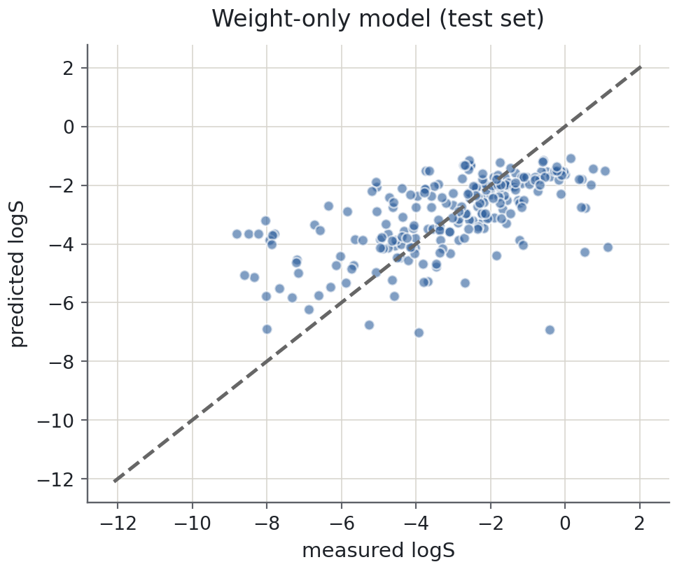
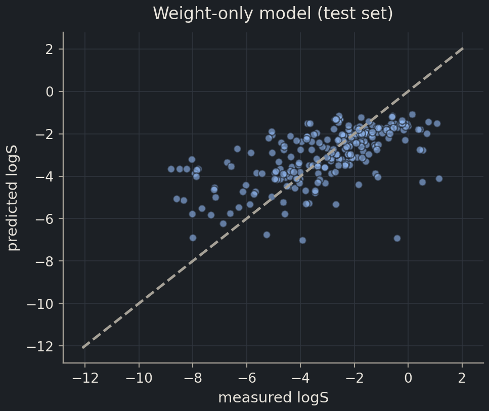
Fit a LinearRegression using onlyMolecular Weight as the feature. Report MAE, RMSE and \(R^2\) on the test set and compare with the baseline and the five-feature model. Then draw its parity plot. What does the single-feature model miss?
Molecular weight alone explains only a modest fraction of the variance: heavier molecules tend to be less soluble, but weight says nothing about polarity. Adding hydrogen-bond donors and polar surface area, both of which favour solubility, is what lifts \(R^2\) to about 0.7. In a parity plot of the weight-only model the points form a broad diagonal cloud with far more scatter than the five-feature version, especially for polar molecules that are much more soluble than their size suggests.
The dataset contains the predictions of Delaney’s original ESOL model in the column ESOL predicted log solubility in mols per litre. Compute the MAE, RMSE and \(R^2\) of those predictions on our test molecules and compare with your linear model. Then think carefully: is this a fair comparison? What might Delaney’s model have seen that ours did not?
SolutionShow solutionHide solution
delaney_pred = esol.loc[X_test.index, "ESOL predicted log solubility in mols per litre"]pd.Series( {"MAE": mean_absolute_error(y_test, delaney_pred),"RMSE": root_mean_squared_error(y_test, delaney_pred),"R2": r2_score(y_test, delaney_pred), }).round(3)
MAE     0.708
RMSE    0.956
R2      0.807
dtype: float64
Delaney’s model is better on every metric. Two caveats make the comparison less clean than it looks:
Different features. ESOL used the calculated octanol–water partition coefficient (clogP), which is strongly related to solubility, as well as molecular weight, rotatable bonds and aromatic proportion. Our five descriptors do not include a lipophilicity term, so part of the gap is the feature set, not the method.
Possible leakage. Delaney fitted his model on (a large part of) this very dataset. Our “test” molecules were therefore probably in his training set, which flatters his numbers in exactly the way this episode warns about. We cannot tell from the file which molecules he held out, so the honest conclusion is “ESOL does well on these compounds”, not “ESOL generalises better”.
Both caveats resurface in Chapter 6 (QSAR), where feature choice and leakage through similar molecules are the central problems.
Where this is going
Everything in this episode transfers unchanged to the rest of the course. In Part II you will evaluate solubility and toxicity models on scaffold splits, where the test molecules have core structures the model never saw, because a random split overstates how well a QSAR model will do on new chemistry. In Part III the same idea becomes a sequence-identity split for proteins. The baselines, the metrics and the parity plots stay exactly as you learned them here; only the way you choose the test set changes, and episode 2.6 starts that story with GroupKFold.
Key points
Performance on training data is not evidence. Always report metrics on data the model has never seen.
Split once, reproducibly, with train_test_split(…, random_state=42), and keep the test set untouched until the end.
A model that cannot beat a DummyRegressor (or DummyClassifier) has learned nothing useful.
MAE is the typical error in target units; RMSE punishes large errors more; R² says how much variance is explained. Report at least two of them.
Metrics summarise, plots explain. A parity plot and a residual plot show where a model goes wrong.