1.2 NumPy arrays

35 min of teaching20 min of exercisesbeginner

Questions this episode answers

Why does scientific Python use arrays instead of lists, and what do I gain?
How do I pick out the rows, columns or readings I want from a grid of numbers?
What does it mean that NumPy is ‘vectorised’, and how much faster is it really?
How do I get random numbers that are the same every time I run the notebook?
What is the X / y convention that every model in this course expects?

What you will be able to do

Create arrays, read their dtype and shape, and index and slice them in one and two dimensions.
Select elements with boolean masks built from comparisons combined with & and |.
Replace a Python loop with vectorised arithmetic and explain the speed-up you measure.
Use broadcasting to subtract a row of column means from a matrix, and aggregate along axis=0 or axis=1.
Draw reproducible random numbers from np.random.default_rng(42) and solve a small linear system with np.linalg.solve.
Lay out a dataset as a feature matrix X of shape (n_samples, n_features) and a target vector y.

A plate reader has just handed you a grid of absorbance readings: 96 wells, each measured every two minutes for an hour. That is about 3,000 numbers, and the questions you want to ask are all whole-grid questions. Which well reacted fastest? What is the mean of the blanks at each time point? Subtract the blank from everything. With lists you would write a loop for each question. With a NumPy array each one is a line, and it runs in compiled code. NumPy is the layer underneath pandas, matplotlib and scikit-learn, so the ideas here, shapes, axes, masks and broadcasting, come back in every later episode.

From lists to arrays

Build an array from a list with np.array. Two attributes tell you what you have: the dtype, the single data type shared by every element, and the shape, the size along each dimension.

import numpy as np

masses_mg = np.array([12.4, 9.8, 15.1])
masses_mg, masses_mg.dtype, masses_mg.shape

(array([12.4,  9.8, 15.1]), dtype('float64'), (3,))

Three floats, 64-bit, in a one-dimensional array of length 3. The shape is a tuple even in one dimension, hence (3,). Unlike a list, an array holds one type only: mix an integer and a float and NumPy promotes everything to float; mix a string in and everything becomes text, which is rarely what you wanted.

The pay-off is arithmetic that applies to the whole array at once:

molar_mass = 18.015
volume_L = 0.250

masses_mg / molar_mass / volume_L      # mmol/L, for every sample

array([2.75326117, 2.17596447, 3.35276159])

No loop. The expression reads like the formula on the page, and the result is a new array of the same shape. This is the pattern from episode 1.1’s comprehension, generalised to any arithmetic and running far faster.

Two-dimensional arrays come from nested lists. Here is a small piece of that plate: four wells, five time points, absorbance at 405 nm.

plate = np.array([
    [0.052, 0.131, 0.209, 0.288, 0.365],   # well A1
    [0.049, 0.102, 0.158, 0.211, 0.263],   # well A2
    [0.055, 0.058, 0.061, 0.063, 0.066],   # well A3, no enzyme
    [0.050, 0.149, 0.247, 0.348, 0.447],   # well A4
])
plate.shape, plate.ndim

((4, 5), 2)

Biologist's corner

This is how every plate-reader export looks once loaded: one row per well, one column per time point (or per wavelength, or per replicate). Keeping the data as a 2-D array rather than 96 separate lists means “the blank at each time point” is plate[2], “every well at t = 0” is plate[:, 0], and “subtract the blank from every well” is one subtraction. A 384-well plate is the same code with a different shape.

Indexing and slicing

Indexing follows episode 1.1: positions start at 0, slices are half-open. In two dimensions you give a row index and a column index, separated by a comma.

plate[0, 4]        # well A1, last time point

np.float64(0.365)

A bare colon means “everything along this axis”, which is how you take a whole row or column:

plate[2], plate[:, 0]

(array([0.055, 0.058, 0.061, 0.063, 0.066]),
 array([0.052, 0.049, 0.055, 0.05 ]))

plate[2] is the third row (the blank), a 1-D array of five readings. plate[:, 0] is the first column, a 1-D array of four readings at \(t = 0\). Slices combine freely: plate[:2, 1:3] is the top two wells at time points 1 and 2, a 2×2 block.

Common mistake

Slices are views, not copies

first_two = plate[:2] does not copy the data. Writing first_two[0, 0] = 0 changes plate too. This is deliberate (copying a million-element array for every slice would be wasteful), but it surprises everyone once. Use plate[:2].copy() when you intend to modify the piece independently.

Boolean masks

Comparing an array with a number gives an array of True/False of the same shape, a boolean mask. Indexing with a mask keeps the elements where it is True.

final = plate[:, -1]                 # absorbance at the last time point
reacted = final > 0.1
final, reacted, final[reacted]

(array([0.365, 0.263, 0.066, 0.447]),
 array([ True,  True, False,  True]),
 array([0.365, 0.263, 0.447]))

Three of the four wells rose above 0.1; the blank did not. Because True counts as 1, reacted.sum() is the number of wells that reacted and reacted.mean() is the fraction. To combine conditions use & (and), | (or) and ~ (not), each condition in its own parentheses:

(final > 0.1) & (final < 0.4)

array([ True,  True, False, False])

Common mistake

and is not &

(final > 0.1) and (final < 0.4) raises ValueError: The truth value of an array with more than one element is ambiguous. Python’s and wants a single True or False; an array of them is neither. Use & and |, and keep the parentheses: & binds tighter than >, so final > 0.1 & final < 0.4 is parsed as final > (0.1 & final) < 0.4, which is nonsense.

Vectorisation: the loop you no longer write

Here is the experiment that justifies NumPy. Take a million absorbance readings, convert each to a concentration with the Beer–Lambert law, \(c = A / (\varepsilon \ell)\), once with a Python loop and once as an array expression, and time both with time.perf_counter().

Predict before you run

Before you run the cell: how many times faster do you expect the array version to be? Two times? Ten? A thousand? Write your guess down.

import time

rng = np.random.default_rng(42)
absorbance = rng.uniform(0.05, 1.5, size=1_000_000)
epsilon, path_cm = 6220.0, 1.0            # NADH at 340 nm, L/(mol cm)

t0 = time.perf_counter()
conc_loop = [a / (epsilon * path_cm) for a in absorbance]
t1 = time.perf_counter()
conc_array = absorbance / (epsilon * path_cm)
t2 = time.perf_counter()

print(f"loop:  {t1 - t0:.3f} s    array: {t2 - t1:.4f} s    "
      f"speed-up: about {(t1 - t0) / (t2 - t1):.0f}x")

loop:  0.588 s    array: 0.0604 s    speed-up: about 10x

The exact number depends on your machine (and on whatever else it is doing), but the array version is reliably tens to hundreds of times faster. This is vectorisation: instead of Python visiting each element, checking its type and performing one operation, NumPy hands the whole block of 64-bit floats to a compiled loop. The code is also shorter and says what you compute rather than how to iterate, which is why the rest of this course almost never loops over data.

The rule of thumb: if you are writing for over the elements of an array, stop and look for the array expression. Comparisons, arithmetic, np.log10, np.exp, np.sqrt and friends all apply element-wise.

Broadcasting

Arithmetic between two arrays of the same shape is element-wise. Arithmetic between arrays of different shapes works when NumPy can stretch one to match the other, a rule called broadcasting. The most useful case is subtracting one row from every row of a matrix.

Take the descriptors of four molecules, three features each: molecular weight in g/mol, number of rings, and polar surface area in Å². Column means come from axis=0:

X = np.array([
    [180.2, 1, 90.2],     # glucose
    [ 78.1, 1,  0.0],     # benzene
    [ 46.1, 0, 20.2],     # ethanol
    [194.2, 2, 61.8],     # caffeine
])
means = X.mean(axis=0)
means

array([124.65,   1.  ,  43.05])

X has shape (4, 3) and means has shape (3,). Subtracting them centres every column at zero:

X_centred = X - means
X_centred.round(1)

array([[ 55.6,   0. ,  47.2],
       [-46.6,   0. , -43. ],
       [-78.5,  -1. , -22.8],
       [ 69.6,   1. ,  18.8]])

In words, NumPy lines the shapes up from the right: (4, 3) against (3,). The trailing dimensions match (3 and 3). The leading dimension is missing from means, so NumPy treats it as 1 and stretches it to 4, as if means were copied into four identical rows. No copy is actually made; the arithmetic simply reuses the same row. The same rule explains the simplest case of all, X * 2: a scalar has no dimensions, so it is stretched to every element.

Two shapes are compatible when, reading from the right, every pair of dimensions is either equal or one of them is 1. (4, 3) with (3,) works. (4, 3) with (4,) does not: 3 against 4, neither is 1. To subtract a per-row value, such as each well’s reading at \(t = 0\), you need the row values as a column of shape (4, 1):

baseline = plate[:, [0]]           # shape (4, 1), not (4,)
(plate - baseline).round(3)

array([[0.   , 0.079, 0.157, 0.236, 0.313],
       [0.   , 0.053, 0.109, 0.162, 0.214],
       [0.   , 0.003, 0.006, 0.008, 0.011],
       [0.   , 0.099, 0.197, 0.298, 0.397]])

Indexing with a list [0] instead of the integer 0 keeps the dimension, which is exactly what broadcasting needs. plate[:, 0:1] and plate[:, 0][:, np.newaxis] do the same thing.

Maths corner

A 1-D array is a vector in \(\mathbb{R}^n\), a 2-D array is a matrix in \(\mathbb{R}^{m \times n}\), and element-wise operations are the Hadamard operations. Broadcasting a row vector \(\mathbf{m}^\top\) across a matrix \(X\) computes \(X - \mathbf{1}\mathbf{m}^\top\), the outer product of the all-ones column with the row, without forming it. The same mechanism gives outer operations for free: for column vector \(\mathbf{a}\) of shape \((n, 1)\) and row vector \(\mathbf{b}\) of shape \((1, k)\), a * b is the outer product \(\mathbf{a}\mathbf{b}^\top\) and a - b is the matrix of all pairwise differences, the first step of every distance computation in Part II. The matrix product is a different operation, written @, below.

Aggregating along an axis

sum, mean, std, min, max, argmax and their relatives all take an axis argument. The axis is the dimension that disappears: axis=0 runs down the rows and leaves one number per column; axis=1 runs across the columns and leaves one number per row. With no axis the whole array collapses to one number.

print("per time point (axis=0):", plate.mean(axis=0).round(3))
print("per well       (axis=1):", plate.mean(axis=1).round(3))
print("overall                :", plate.mean().round(3))

per time point (axis=0): [0.052 0.11  0.169 0.228 0.285]
per well       (axis=1): [0.209 0.157 0.061 0.248]
overall                : 0.169

The first line averages the four wells at each time point (five numbers); the second averages the five readings of each well (four numbers). A quick way to remember: the result’s shape is the input shape with the named axis removed, so (4, 5) with axis=0 gives (5,).

rates = (plate[:, -1] - plate[:, 0]) / 8.0      # absorbance per minute over 8 min
fastest = rates.argmax()
print(f"rates: {rates.round(4)}   fastest well: row {fastest}")

rates: [0.0391 0.0268 0.0014 0.0496]   fastest well: row 3

argmax returns the position of the maximum, which is how you get from “which value is largest” to “which well”.

Common mistake

Standard deviation: NumPy divides by n

np.std computes the population standard deviation (dividing by \(n\)). pandas and most statistics packages divide by \(n - 1\) (the sample standard deviation). On three replicates the difference is large. If you want the sample version from NumPy, pass ddof=1.

Random numbers you can reproduce

Simulations, bootstrapping, shuffling data before a split: all need random numbers, and all must give the same answer tomorrow. NumPy’s random number generator is an object you create once with a seed and then draw from:

rng = np.random.default_rng(42)

print("normal  :", rng.normal(loc=100, scale=5, size=4).round(1))   # mean 100, sd 5
print("uniform :", rng.uniform(0, 1, size=3).round(3))
print("integers:", rng.integers(1, 7, size=6))                       # dice: 1..6, upper bound excluded
print("choice  :", rng.choice(["Adelie", "Chinstrap", "Gentoo"], size=4))

normal  : [101.5  94.8 103.8 104.7]
uniform : [0.094 0.976 0.761]
integers: [5 5 4 1 6 3]
choice  : ['Chinstrap' 'Chinstrap' 'Adelie' 'Gentoo']

The seed, 42 by convention, fixes the entire sequence. Re-create the generator with the same seed and you get the same numbers in the same order; so does your colleague, and so does this website when it is rebuilt. That is what makes “I shuffled the data and got RMSE 0.93” a statement someone else can check. Draw everything from the one generator rather than creating a new one per cell, and avoid the older global-state functions (np.random.rand and the module-level seed) that you will see in old tutorials: any cell or library can reset that shared state behind your back.

A thousand replicate measurements of a 100 µM standard, with 5% instrument noise, look like this:

import matplotlib.pyplot as plt

measurements = rng.normal(loc=100, scale=5, size=1000)

fig, ax = plt.subplots()
ax.hist(measurements, bins=30)
ax.set(xlabel="measured concentration (µM)", ylabel="count",
       title="1000 draws from normal(100, 5)")
plt.show()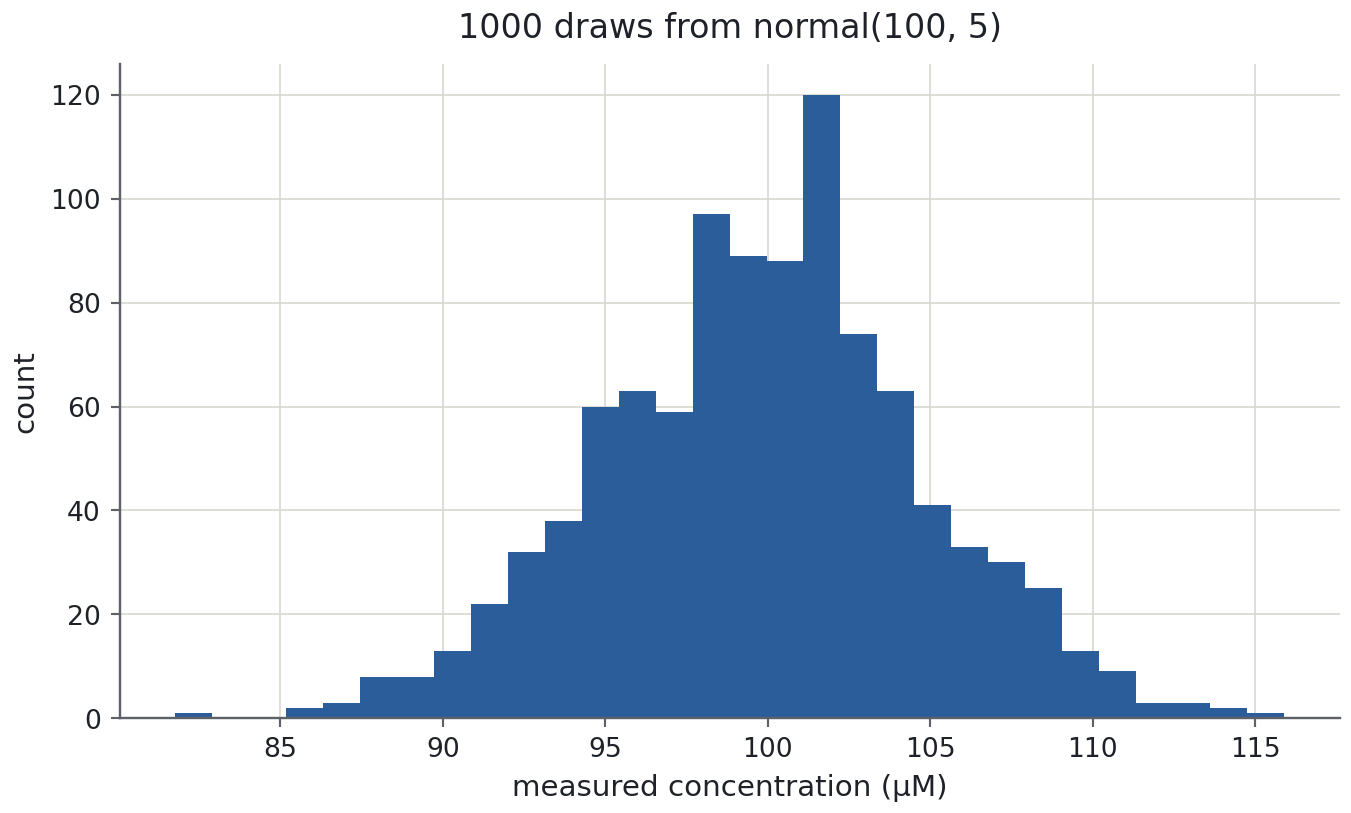

Histogram of 1000 simulated concentration measurements drawn from a normal distribution with mean 100 micromolar and standard deviation 5. The bars form a bell shape centred on 100, extending from about 82 to 116.

The histogram is the bell curve you expect, centred on 100 with almost everything within 15 µM (three standard deviations). Episode 1.4 covers the plotting commands; for now notice the shape of the code: fig, ax = plt.subplots(), draw on ax, label with units, plt.show().

Matrices: `@` and solving a linear system

* multiplies element by element. The matrix product is @. You need it rarely in this chapter and constantly from Chapter 2 on, so here is one concrete use: mixing stock solutions.

You have two stock solutions. Stock 1 is 50 mM Tris and 10 mM NaCl; stock 2 is 10 mM Tris and 100 mM NaCl. You want one litre of buffer containing 20 mmol Tris and 40 mmol NaCl, topped up with water. Which volumes \(v_1\) and \(v_2\) (in litres) of each stock do you need? Each solute gives one equation:

\[ 50\,v_1 + 10\,v_2 = 20, \qquad 10\,v_1 + 100\,v_2 = 40 . \]

In matrix form that is \(A\mathbf{v} = \mathbf{b}\), with \(A\) holding the stock concentrations (one row per solute, one column per stock) and \(\mathbf{b}\) the target amounts:

A = np.array([[50.0, 10.0],
              [10.0, 100.0]])
b = np.array([20.0, 40.0])

v = np.linalg.solve(A, b)
print(f"stock 1: {v[0]:.3f} L   stock 2: {v[1]:.3f} L   water: {1 - v.sum():.3f} L")
print("check A @ v =", A @ v)

stock 1: 0.327 L   stock 2: 0.367 L   water: 0.306 L
check A @ v = [20. 40.]

About 327 mL of stock 1, 367 mL of stock 2 and water to a litre. A @ v reproduces the target amounts, which is the test that you solved the right system. With ten solutes and ten stocks the code is identical; only the shapes change. Never invert a matrix to solve a system (np.linalg.inv(A) @ b): solve is faster and numerically safer, and in Chapter 2 the same function fits a linear regression through the normal equation.

The X / y convention

Note

X is (n_samples, n_features); y is (n_samples,)

Every dataset in this course, and every scikit-learn estimator, uses one layout, the X / y convention:

X is a 2-D array with one row per sample (a molecule, a penguin, a patient) and one column per feature (a descriptor, a measurement). Its shape is (n_samples, n_features).
y is a 1-D array with one target per sample, the label you want to predict. Its shape is (n_samples,), and its length equals the number of rows of X.

The four-molecule descriptor matrix above is already an X. Add the quantity you want to predict, say measured solubility as logS in log₁₀(mol/L), and you have a complete supervised-learning dataset:

y = np.array([0.74, -1.64, 1.10, -0.88])   # logS: glucose, benzene, ethanol, caffeine

print("X:", X.shape, "  y:", y.shape)
print("features of molecule 3 (caffeine):", X[3])
print("all molecular weights:            ", X[:, 0])

X: (4, 3)   y: (4,)
features of molecule 3 (caffeine): [194.2   2.   61.8]
all molecular weights:             [180.2  78.1  46.1 194.2]

X[i] is one sample, X[:, j] is one feature across all samples, and X.mean(axis=0) is the vector of feature means. Keep this picture: it is what axis=0 means for the rest of the course.

Exercises

Exercise★☆☆

Shapes and axes

Without running code, write down the shape of each result: plate[1], plate[:, 1], plate[1:3, :2], plate.sum(axis=0), plate.sum(axis=1), plate > 0.1. Then check your answers.

SolutionShow solution

for name, value in [
    ("plate[1]", plate[1]),
    ("plate[:, 1]", plate[:, 1]),
    ("plate[1:3, :2]", plate[1:3, :2]),
    ("plate.sum(axis=0)", plate.sum(axis=0)),
    ("plate.sum(axis=1)", plate.sum(axis=1)),
    ("plate > 0.1", plate > 0.1),
]:
    print(f"{name:<20}{str(value.shape):>8}   dtype {value.dtype}")

plate[1]                (5,)   dtype float64
plate[:, 1]             (4,)   dtype float64
plate[1:3, :2]        (2, 2)   dtype float64
plate.sum(axis=0)       (5,)   dtype float64
plate.sum(axis=1)       (4,)   dtype float64
plate > 0.1           (4, 5)   dtype bool

A single integer index removes that axis ((4, 5) becomes (5,) for a row, (4,) for a column); a slice keeps it, so plate[1:3, :2] stays 2-D. Aggregating along an axis removes it: axis=0 leaves one number per column, (5,); axis=1 one per row, (4,). A comparison keeps the shape and changes the dtype to bool.

Exercise★☆☆

Debug this

A colleague wants the mean of the readings that fall between 90 and 110 µM. Neither attempt works. Find the bug in each, then write a version that does.

readings = rng.normal(loc=100, scale=5, size=1000)

# attempt 1
good = []
for r in readings:
    if r > 90 and r < 110:
        good.append(r)
print(good.mean())

# attempt 2
good = readings[readings > 90 and readings < 110]
print(good.mean())

SolutionShow solution

Attempt 1 builds a Python list, and lists have no .mean() method, so the last line raises AttributeError: 'list' object has no attribute 'mean'. The loop itself is fine (comparing one float with and is legal), just slow. np.mean(good) would rescue it, but the better fix is to drop the loop.

Attempt 2 uses and on two arrays, which raises ValueError: The truth value of an array with more than one element is ambiguous. Element-wise “and” is &, and each comparison needs parentheses.

readings = rng.normal(loc=100, scale=5, size=1000)

mask = (readings > 90) & (readings < 110)
print(f"{mask.sum()} readings kept, mean {readings[mask].mean():.2f} µM")

946 readings kept, mean 99.74 µM

About 95% of draws fall within two standard deviations of the mean, so roughly 950 readings are kept, and their mean is close to 100 because the window is symmetric.

Exercise★★☆

Normalise the plate

For each well in plate, subtract its own reading at \(t = 0\) (use broadcasting with a (4, 1) column, not a loop), then divide every well by the final reading of the fastest well so that the largest value on the plate is 1. Report the shape at each step and the normalised final readings.

SolutionShow solution

zeroed = plate - plate[:, [0]]                    # (4, 5) - (4, 1)
fastest = zeroed[:, -1].argmax()
normalised = zeroed / zeroed[fastest, -1]         # (4, 5) / scalar

print("zeroed:", zeroed.shape, " normalised:", normalised.shape)
print("final readings, normalised:", normalised[:, -1].round(3))

zeroed: (4, 5)  normalised: (4, 5)
final readings, normalised: [0.788 0.539 0.028 1.   ]

plate[:, [0]] keeps the column dimension, so its shape (4, 1) broadcasts against (4, 5) by stretching along the time axis: every reading in a row has that row’s \(t = 0\) value subtracted. Had you written plate[:, 0] (shape (4,)) NumPy would have tried to line 4 up against 5 and failed. Dividing by a scalar broadcasts to every element. Well A4 (row 3) is the fastest and lands exactly at 1; the blank stays near 0.

Exercise★★★

A calibration line by linear algebra

A Beer–Lambert calibration measured absorbance at five known concentrations. Fit the straight line \(A = \theta_0 + \theta_1 c\) by solving the normal equations \((X^\top X)\,\boldsymbol{\theta} = X^\top \mathbf{y}\) with np.linalg.solve, where X has a column of ones (for the intercept) and a column of concentrations. Compare with np.linalg.lstsq(X, y, rcond=None)[0], and use the fitted line to estimate the concentration of a sample with absorbance 0.40.

conc = np.array([0.0, 0.1, 0.2, 0.4, 0.8])          # mM
absorb = np.array([0.023, 0.135, 0.278, 0.529, 1.000])

SolutionShow solution

conc = np.array([0.0, 0.1, 0.2, 0.4, 0.8])
absorb = np.array([0.023, 0.135, 0.278, 0.529, 1.000])

X_cal = np.column_stack([np.ones(len(conc)), conc])   # shape (5, 2)
theta = np.linalg.solve(X_cal.T @ X_cal, X_cal.T @ absorb)
theta_lstsq = np.linalg.lstsq(X_cal, absorb, rcond=None)[0]

print("normal equations:", theta.round(4))
print("lstsq           :", theta_lstsq.round(4))
print(f"sample at A = 0.40: {(0.40 - theta[0]) / theta[1]:.3f} mM")

normal equations: [0.0246 1.228 ]
lstsq           : [0.0246 1.228 ]
sample at A = 0.40: 0.306 mM

X_cal is an X in the sense of this episode: five samples, two features (a constant and the concentration), and absorb is the y. X.T @ X is 2×2 and X.T @ y has two entries, so solve returns the intercept and the slope that minimise the squared vertical distances to the line. lstsq gives the same answer by a numerically more careful route and is what you should use in practice; the point of doing it by hand once is that episode 2.2 fits linear regression with exactly this equation, and LinearRegression().fit(X, y) is this cell wrapped in a class.

Where this is going

The feature matrix X and target y you built here are the input to every model in the course: in Chapter 2 train_test_split(X, y) carves them into training and test sets and LinearRegression().fit(X, y) solves the same normal equations as the last exercise, at scale. Broadcasting is how feature scaling works ((X - X.mean(axis=0)) / X.std(axis=0)), how distances between molecules are computed in Part II, and how a whole gene-expression matrix is normalised in Part III. The next episode, 1.3, puts labels on the rows and columns of an array and calls the result a DataFrame.

Key points

An array holds one data type in a fixed shape; that is what makes whole-array arithmetic fast and lets shape tell you what you are holding.
a[i, j] picks an element, a[:, j] a column, a[i] a row; slices are views, so writing to a slice changes the original.
A boolean mask a[a > 0] selects elements; combine conditions with & and | in parentheses, never and/or.
Vectorised code is tens to hundreds of times faster than the equivalent loop, and usually shorter and clearer.
Broadcasting stretches the smaller array along missing or length-1 axes; X - X.mean(axis=0) centres every column.
axis=0 collapses rows (one result per column); axis=1 collapses columns (one result per row).
Create one rng = np.random.default_rng(42) and draw everything from it; a fixed seed makes results reproducible.
Features live in X, shape (n_samples, n_features); targets in y, shape (n_samples,). Every estimator in the course expects this.

1.2 NumPy arrays

Questions this episode answers

What you will be able to do

From lists to arrays

Indexing and slicing

Boolean masks

Vectorisation: the loop you no longer write

Broadcasting

Aggregating along an axis

Random numbers you can reproduce

Matrices: @ and solving a linear system

The X / y convention

Exercises

Where this is going

Key points

Matrices: `@` and solving a linear system