2.1 What is machine learning?

25 min of teaching10 min of exercisesbeginner

Questions this episode answers

What does it mean for a computer to learn from data, and how is that different from fitting a curve?
When is a question a regression, a classification or an unsupervised problem, and when is it not a machine-learning problem at all?
Where does machine learning genuinely help in chemistry and biology, and where does it quietly fail?

What you will be able to do

Classify a scientific question as regression, classification, unsupervised learning or none of these.
Describe a model as a function \(f(x;\theta)\) whose parameters are chosen by minimising a loss on training data.
Name the features and labels of a concrete dataset and arrange them in the X / y convention.
Recognise underfitting and overfitting in a fitted curve and explain why generalisation, not training fit, is the goal.
List the conditions (tiny data, distribution shift, label noise, confounding) under which a model’s predictions should not be trusted.

In episode 1.5 you explored 1,128 small molecules with measured aqueous solubility and saw that heavier molecules tend to be less soluble. Now a colleague proposes a 1,129th molecule. Nobody has made it, so nobody has measured it. Can the 1,128 measurements tell you, before anyone spends a week in the lab, roughly how soluble it will be?

That question, predict a property of something new from examples of things already measured, is the whole of machine learning in one sentence. This episode gives you the vocabulary to state such questions precisely, a mental picture of what a model is, and a feel for when the answer will be worthless.

Learning from examples

In ordinary programming you write the rule and the computer applies it: to convert grams to moles you write mass / molar_mass, and the rule is right by construction. In machine learning you have no rule, only examples, 1,128 pairs of (molecule, solubility). The computer’s job is to find a rule that reproduces the examples and, with luck, works on the next molecule too.

A model is that candidate rule, written as a function:

\[ \hat{y} = f(x;\, \theta) \]

Here \(x\) is what you know about the sample, \(\hat{y}\) is the prediction (the hat marks a guess rather than a measurement), and \(\theta\) (theta) are the parameters: the numbers inside the function that the data get to choose. The simplest model for solubility is a straight line,

\[ \hat{y} = \theta_0 + \theta_1 \cdot \text{molecular weight}, \]

with an intercept \(\theta_0\) and a slope \(\theta_1\). Learning means choosing them so that the line passes close to the measured points. If that sounds like curve fitting, it is: most of this chapter builds on the resemblance. What changes is the ambition (hundreds of inputs, functions far more flexible than a line) and, above all, the question. A curve fitter asks how well does this line describe my data? A machine learner asks how well will it describe data I have not seen?

For programmers

Think of it as programming by example. The model is a function whose signature you choose (inputs: molecular descriptors; output: a solubility) but whose body is filled in by an optimiser rather than by you. The parameters \(\theta\) are the function’s constants, training is the search over those constants, and the loss function below is the test suite the search tries to satisfy, except that a loss is a number you can only make smaller, never pass.

Chemist's corner

You have met one-feature linear models before. A Hammett plot puts \(\log(k/k_0)\) against the substituent constant \(\sigma\) and reads the reaction constant \(\rho\) off the slope: a model \(f(\sigma;\rho)\) with one parameter, fitted to examples. Quantitative structure–activity relationships (QSAR) extend the idea to many descriptors at once; in this episode’s vocabulary, QSAR is supervised regression, and Part II is largely about doing it well.

Three kinds of problem

The solubility examples come with answers: each molecule has a measured value. Learning from examples that carry the correct answer is supervised learning, and it splits into two families by the type of answer.

regression: the answer is a number on a continuous scale. Solubility in log units, melting point in °C, binding free energy in kcal/mol.
classification: the answer is a category. Toxic or non-toxic, active or inactive against a target, benign or malignant tumour.

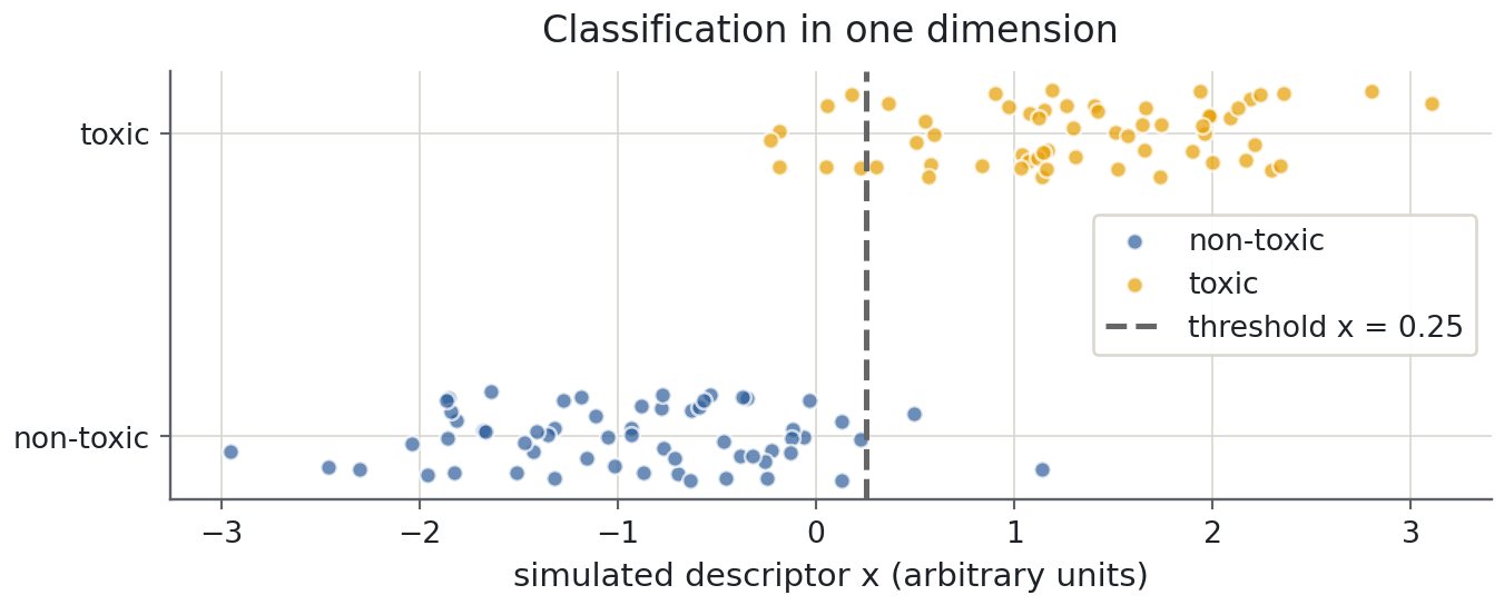
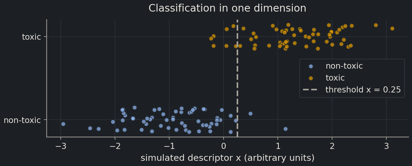
The two are closer than they look. The figure shows a classification problem with a single simulated descriptor \(x\) for sixty non-toxic and sixty toxic compounds. The classes overlap, so no rule is perfect, but a threshold on \(x\) separates most of them, and the position of that threshold is a parameter chosen from the data, exactly as a slope is.

import matplotlib.pyplot as plt
import numpy as np

rng = np.random.default_rng(42)
non_toxic = rng.normal(-1.0, 1.0, 60)   # simulated descriptor values, class 0
toxic = rng.normal(1.5, 1.0, 60)        # simulated descriptor values, class 1
threshold = 0.25

fig, ax = plt.subplots(figsize=(7, 2.8))
ax.scatter(non_toxic, rng.uniform(-0.15, 0.15, 60), alpha=0.7, label="non-toxic")
ax.scatter(toxic, 1 + rng.uniform(-0.15, 0.15, 60), alpha=0.7, label="toxic")
ax.axvline(threshold, linestyle="--", color="0.4", label=f"threshold x = {threshold}")
ax.set(xlabel="simulated descriptor x (arbitrary units)", yticks=[0, 1],
       yticklabels=["non-toxic", "toxic"], title="Classification in one dimension")
ax.legend(loc="center right")
plt.show()

A one-dimensional classification example. Sixty non-toxic compounds are drawn as points on a lower row and sixty toxic compounds on an upper row, each spread along a simulated descriptor x. The non-toxic cloud is centred near x = -1 and the toxic cloud near x = 1.5; they overlap between about 0 and 1. A dashed vertical line at x = 0.25 marks a threshold that classifies most compounds correctly.

Not every dataset comes with answers. A sequencing run gives the expression of 20,000 genes in each of 500 tumour samples; a virtual library gives 200 molecular descriptors for each of 100,000 compounds. Nobody has labelled them, and the question is simply what structure is in here? That is unsupervised learning. Two kinds you will meet:

Clustering groups samples that look alike. Clustering the expression profiles of tumour samples can reveal subtypes no pathologist had named.
Dimensionality reduction, most often principal component analysis (PCA), compresses hundreds of correlated descriptors into two or three axes that keep most of the variation, so that you can see where a compound library sits in chemical space.

Some scientific questions are not machine-learning problems at all, and recognising them is part of the skill. Computing the exact mass of C₈H₁₀N₄O₂ is a deterministic calculation. Deciding whether a gene is expressed more in treated than in control samples is a hypothesis test about this experiment, not a prediction about the next one.

Biologist's corner

Differential expression analysis and a predictive model can run on the same data and answer different questions. Differential expression explains: which genes differ between conditions, with a p-value each. A classifier predicts: does the profile of a new, unseen sample let you call its condition? A gene can differ significantly on average yet be useless for prediction because the conditions overlap too much, and a model can predict well using genes that are not individually significant. Keep explaining and predicting apart in your head; a surprising number of published models muddle them.

Question	Kind	Output
How soluble will this molecule be?	supervised, regression	a number (logS)
Will this compound inhibit the enzyme?	supervised, classification	a category (yes / no)
Which of these tumours resemble each other?	unsupervised, clustering	group memberships
What are the main axes of variation in this library?	unsupervised, dimensionality reduction	a few summary coordinates
What is the exact mass of this formula?	not machine learning	a calculation

Features, labels and the X / y convention

The things you know about each sample are its features; the thing you want to predict is its label (in regression also called the target). Almost every tool you will use expects them in one layout, the X / y convention: a two-dimensional table X with one row per sample and one column per feature, and a one-dimensional y with one label per row, in the same order.

Here it is for the solubility data, with five descriptors that come with the file as features and measured logS as the label.

from pathlib import Path

import pandas as pd

ESOL_URL = "https://deepchemdata.s3-us-west-1.amazonaws.com/datasets/delaney-processed.csv"
path = Path("data/esol.csv")
esol = pd.read_csv(path if path.exists() else ESOL_URL)

features = [
    "Molecular Weight",
    "Number of H-Bond Donors",
    "Number of Rings",
    "Number of Rotatable Bonds",
    "Polar Surface Area",
]
X = esol[features]
y = esol["measured log solubility in mols per litre"]
X.head(3)

index	Molecular Weight	Number of H-Bond Donors	Number of Rings	Number of Rotatable Bonds	Polar Surface Area
0	457.432	7	3	7	202.32
1	201.225	1	2	2	42.24
2	152.237	0	0	4	17.07

print(f"X: {X.shape[0]} samples × {X.shape[1]} features    y: {y.shape[0]} labels")

X: 1128 samples × 5 features    y: 1128 labels

The shapes are the first thing to check in any project: X has as many rows as y has entries, in the same order, so that row 17 of X describes the molecule whose solubility is entry 17 of y. Sort one without the other and every model you fit afterwards is nonsense, with no error message.

Common mistake

The label is in the table too

The ESOL file also contains Delaney’s own predicted solubilities. It is tempting to add that column to X; it is, after all, a number per molecule. But it was computed from the measured values you are trying to predict, so a model using it would be copying the answer. Whether a column is a legitimate feature is a judgement about how the data were produced, not about the file layout; episode 2.6 is devoted to the ways this goes wrong.

A loss turns “better” into a number

Two people draw two different lines through the solubility data. Who is right? To decide you need a loss function: a single number that says how badly a model’s predictions miss the labels, with zero meaning perfect. For regression the standard choice is the mean squared error (MSE): take the difference between each measured value and its prediction, square it (so that misses above and below both count, and large misses count a lot), and average over the \(n\) samples:

\[ \mathrm{MSE}(\theta) = \frac{1}{n}\sum_{i=1}^{n}\bigl(y_i - f(x_i;\theta)\bigr)^2 . \]

For classification a squared difference makes no sense, because “toxic minus non-toxic” is not a number. The simplest loss is the fraction of samples put in the wrong class. In practice models predict a probability of each class, and the training loss (the log loss) punishes confident wrong answers far more than hesitant ones; episode 2.5 builds this up properly.

The loss is written as a function of \(\theta\) on purpose. The data are fixed; the parameters are what you can change; training is the search for the \(\theta\) that makes the loss as small as possible on the training data. Here are two candidate lines for logS against molecular weight, scored by their MSE.

Predict before you run

Line A ignores molecular weight and predicts the mean logS for every molecule (slope 0). Line B has intercept −0.4 and slope −0.013 per g/mol. Which will have the smaller MSE, and by roughly what factor? Write your guess down before running the cell.

x = esol["Molecular Weight"]


def mse(theta0, theta1, x, y):
    """Mean squared error of the line theta0 + theta1 * x on the data (x, y)."""
    y_hat = theta0 + theta1 * x
    return np.mean((y - y_hat) ** 2)


print(f"line A (flat, at the mean): MSE = {mse(y.mean(), 0.0, x, y):.3f}")
print(f"line B (sloping):           MSE = {mse(-0.4, -0.013, x, y):.3f}")

line A (flat, at the mean): MSE = 4.391
line B (sloping):           MSE = 2.592

Line B misses by about 40% less, in squared log units, so molecular weight carries real information about solubility. The numbers matter less than the move: which line is better has become which number is smaller, a question a computer can answer by trying many values of \(\theta\). How it searches efficiently, with an exact formula and with gradient descent, is episode 2.2.

Maths corner

Formally, supervised learning is function approximation under uncertainty: you want the \(f\) in a chosen family \(\mathcal{F}\) (all lines, all cubics, all neural networks of a given shape) that minimises the expected loss over the distribution the data come from. You cannot compute that expectation from a sample, so you minimise the average loss on the sample instead. This is empirical risk minimisation, and most of this chapter is a consequence of the gap between the two quantities.

Deep diveEmpirical risk minimisation, stated preciselyShow the maths

Assume the pairs \((x_i, y_i)\) are independent draws from an unknown distribution \(P\) over \(\mathcal{X}\times\mathcal{Y}\). For a loss \(\ell(\hat{y}, y)\) and a function \(f \in \mathcal{F}\), the risk is

\[ R(f) = \mathbb{E}_{(x,y)\sim P}\bigl[\ell(f(x), y)\bigr], \]

and the empirical risk on a sample of size \(n\) is

\[ \hat{R}_n(f) = \frac{1}{n}\sum_{i=1}^{n} \ell(f(x_i), y_i). \]

Training returns \(\hat{f} = \arg\min_{f\in\mathcal{F}} \hat{R}_n(f)\); the quantity you care about is \(R(\hat{f})\). With \(\ell(\hat y, y) = (\hat y - y)^2\) the empirical risk is the MSE above. The two risks differ because \(\hat{R}_n\) is a noisy estimate of \(R\), and because the minimiser of a noisy estimate is biased downwards: you chose \(\hat f\) because it looked good on this sample. The second effect grows with the size of \(\mathcal{F}\), which is the formal content of the next section.

Fitting is not the same as learning

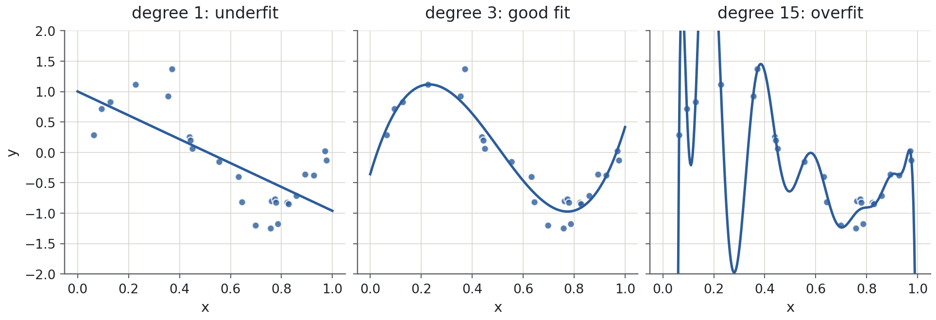
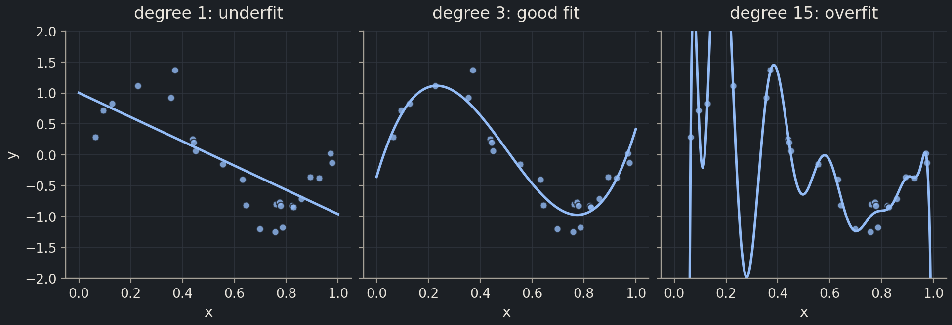
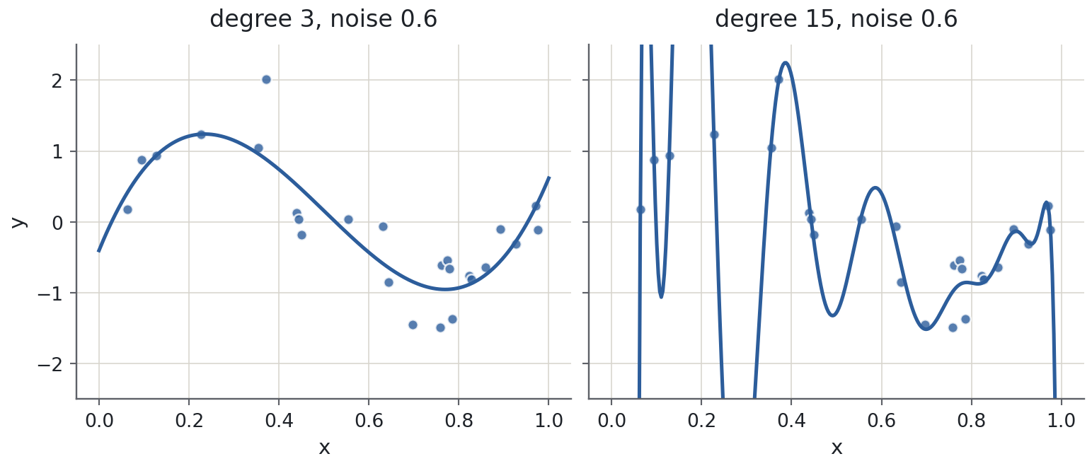
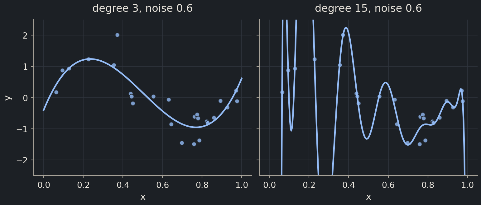
If training means making the loss small, why not use a model flexible enough to make it zero? A small experiment answers the question. The data are 25 points from a sine curve with noise added, standing in for any smooth relationship measured imperfectly. We fit polynomials of degree 1, 3 and 15 to the same points.

rng = np.random.default_rng(42)
x_toy = np.sort(rng.uniform(0, 1, 25))
y_toy = np.sin(2 * np.pi * x_toy) + rng.normal(0, 0.3, 25)
grid = np.linspace(0, 1, 300)

fig, axes = plt.subplots(1, 3, figsize=(10, 3.4), sharey=True)
for ax, degree, verdict in zip(axes, [1, 3, 15], ["underfit", "good fit", "overfit"]):
    poly = np.polynomial.Polynomial.fit(x_toy, y_toy, degree)
    ax.scatter(x_toy, y_toy, alpha=0.8)
    ax.plot(grid, poly(grid))
    ax.set(title=f"degree {degree}: {verdict}", xlabel="x", ylim=(-2, 2))
axes[0].set(ylabel="y")
plt.show()

Three panels showing the same 25 noisy points from a sine curve on the interval 0 to 1, each with a fitted polynomial. Left, degree 1: a straight line that misses the curvature, labelled underfit. Middle, degree 3: a smooth cubic that follows the sine shape closely, labelled good fit. Right, degree 15: a curve that passes through almost every point but swings wildly between them and shoots off the axes near the edges, labelled overfit.

for degree in [1, 3, 15]:
    poly = np.polynomial.Polynomial.fit(x_toy, y_toy, degree)
    print(f"degree {degree:>2}: training MSE = {np.mean((y_toy - poly(x_toy)) ** 2):.4f}")

degree  1: training MSE = 0.2574
degree  3: training MSE = 0.0441
degree 15: training MSE = 0.0098

Read the three panels against the three numbers:

Degree 1 cannot bend, so it misses a shape that is obviously there. Its loss is large and its predictions are systematically wrong: underfitting, a model too simple for the pattern.
Degree 3 follows the sine curve and ignores the scatter around it. It is wrong by about the size of the noise, which is the best any model can do.
Degree 15 has the smallest training loss by far and is the worst model of the three. It has spent its 16 parameters chasing the noise, and between the points, especially beyond the last one, it predicts values no new measurement would ever show: overfitting, a model that has memorised the training data instead of learning the relationship.

The training loss falls steadily with the degree and would keep falling until the curve passed through every point. So the training loss cannot be what you use to choose a model; if it were, the most flexible model would always win. What you want is generalisation: a small error on new points from the same process. That is the only measure of whether a model has learned anything, and it cannot be read off the training data at all. Measuring it honestly is episode 2.3; controlling the flexibility behind the right-hand panel is episode 2.4.

Common mistake

A smaller training error is not a better model

Whenever someone shows you a fit that goes through every point, ask what it predicts between the points and beyond them. The degree-15 curve leaves the plot before \(x\) reaches 0.1. Perfect agreement with the data you have is a warning sign, not a result.

Where machine learning helps, and where it fails

The polynomial experiment used 25 points. Real projects range from a dozen measurements to millions, and the size and character of the data decide whether machine learning is the right tool.

It earns its keep in three situations.

Large datasets. High-throughput screens, public bioactivity databases and sequencing runs hold more samples than a person can look at, with patterns too diffuse to write down as rules. A model with many parameters is harmless when the data can pin every parameter down.
Pattern-rich inputs. A microscopy image, a protein sequence or a mass spectrum is thousands of raw numbers with no obvious equation linking them to the answer. Hand-written rules (“a cell is mitotic if its texture is such-and-such”) fail; learning the rule from labelled examples is the only approach that has worked at scale.
Fast surrogates for slow things. A quantum-chemical energy takes hours per molecule; a synthesis and assay take a week. A model trained on a few thousand completed calculations or experiments can rank a million candidates in seconds, so the expensive step is spent only on the promising ones.

And it fails, usually quietly, in four.

Small data. With thirty measurements even a straight line has uncertain parameters, and anything more flexible overfits as surely as the degree-15 polynomial did. For datasets of dozens, a mechanistic model, a careful statistical analysis or simply more experiments usually beat machine learning.
Distribution shift. A model learns the data it was trained on. Ask it about a new chemical scaffold, cells from a different lab, samples processed with a new kit or patients from another hospital, and it can be confidently wrong, because nothing in the training set resembles the question. In chemistry this is the rule, not the exception: the molecules you most want to predict are the novel ones.
Label noise. If the assay behind the labels is reproducible to ±0.5 log units, no model can be reliably better than that, and one that appears to be has fitted the noise. Know the error of your labels before you judge the error of your model.
Confounded data. Models find the easiest pattern that explains the labels, not the one you intended. If the toxic compounds were measured in one lab and the non-toxic ones in another, or the diseased tissue was imaged on a different microscope, the model learns to detect the lab or the microscope. It will score brilliantly on your data and uselessly on anyone else’s.

None of these is a reason to avoid machine learning. They are the questions to ask before fitting anything: how many samples do I have, how different will the samples I care about be, how noisy are my labels, and what else differs between my classes?

Discussion

A group reports a model that predicts, from structure, whether a compound will be toxic in mice, trained on 180 compounds, 160 of them from a single chemical series. Which of the four failure modes worries you most, and what one extra piece of information would you ask for?

Exercises

Exercise★☆☆

Which kind of problem?

For each question, decide whether it is regression, classification, unsupervised learning or not a machine-learning problem as stated. Say in a few words what the label (if any) is.

Predict the melting point of a compound from its structure.
Decide whether a compound inhibits a kinase at 10 µM.
Group 5,000 tumour samples by their expression profiles when no diagnoses are available.
Compute the exact mass of C₈H₁₀N₄O₂.
Predict whether a protein sequence is secreted from the cell.
Estimate the binding free energy of a ligand to a protein.
Find which of 200 descriptors vary together across a compound library.
Test whether gene X is expressed more in treated than in control samples.
Predict a patient’s blood glucose 30 minutes from now from a sensor trace.
Sort 10,000 microscope images into “cell in mitosis” or “not”.

SolutionShow solution

Regression; label = melting point (°C).
Classification; label = inhibits / does not inhibit. (With the measured IC₅₀ as label it would be regression; the threshold at 10 µM makes it a category.)
Unsupervised (clustering); no label.
Not machine learning: a deterministic calculation from atomic masses.
Classification; label = secreted / not secreted.
Regression; label = free energy (kcal/mol).
Unsupervised (dimensionality reduction, for example PCA); no label.
Not machine learning as stated: a hypothesis test about this experiment. Predicting the treatment status of a new sample from its expression would be classification.
Regression; label = glucose concentration 30 minutes ahead.
Classification; label = mitotic / not mitotic.

Several of these change kind if you change the label. “What do I want to know about the next sample?” is what decides.

Exercise★★☆

Degree and noise

Reuse x_toy from the polynomial figure and generate new noisy y values with noise standard deviation 0.1 and then 0.6 (keep np.random.default_rng(42)). For each noise level fit polynomials of degree 1, 3, 5, 9 and 15 and print the training MSE. Then draw the degree-3 and degree-15 fits at the high noise level. What changes with the noise, and what does not?

SolutionShow solution

def training_mse(degree, y):
    poly = np.polynomial.Polynomial.fit(x_toy, y, degree)
    return np.mean((y - poly(x_toy)) ** 2)


rng = np.random.default_rng(42)
signal = np.sin(2 * np.pi * x_toy)
y_quiet = signal + rng.normal(0, 0.1, 25)
y_noisy = signal + rng.normal(0, 0.6, 25)

degrees = [1, 3, 5, 9, 15]
pd.DataFrame(
    {
        "noise 0.1": [training_mse(d, y_quiet) for d in degrees],
        "noise 0.6": [training_mse(d, y_noisy) for d in degrees],
    },
    index=pd.Index(degrees, name="degree"),
).round(4)

index	noise 0.1	noise 0.6
degree	index	index
1	0.1657	0.4207
3	0.0071	0.1642
5	0.0053	0.1506
9	0.0031	0.1140
15	0.0019	0.0392

fig, axes = plt.subplots(1, 2, figsize=(8, 3.4), sharey=True)
for ax, degree in zip(axes, [3, 15]):
    poly = np.polynomial.Polynomial.fit(x_toy, y_noisy, degree)
    ax.scatter(x_toy, y_noisy, alpha=0.8)
    ax.plot(grid, poly(grid))
    ax.set(title=f"degree {degree}, noise 0.6", xlabel="x", ylim=(-2.5, 2.5))
axes[0].set(ylabel="y")
plt.show()

Two panels showing the same 25 very noisy points from a sine curve. Left: a degree-3 polynomial that still recovers the broad sine shape through the scatter. Right: a degree-15 polynomial that wiggles sharply to pass near individual points and leaves the plot area near both edges.

What does not change: at either noise level the training MSE falls monotonically with degree, because a higher-degree polynomial can always do at least as well as a lower one on the points it is fitted to. What changes: with quiet data the degree-3 fit is already almost perfect and higher degrees gain almost nothing, whereas with noisy data the high-degree fits “gain” a lot of training MSE by chasing scatter that carries no information. The noisier the data, the bigger the gap between fitting and learning, and the more you need a measure of generalisation that does not rely on the training loss.

Exercise★★★

Minimise a loss by hand

Three measurements: \(x = (1, 2, 3)\), \(y = (2, 3, 5)\). Use the one-parameter model \(\hat{y} = \theta x\) (a line through the origin). Write the MSE as an explicit function of \(\theta\), expand it, find the minimising \(\theta\) with a derivative, and check your answer numerically by evaluating the loss on a grid of \(\theta\) values.

SolutionShow solution

The loss is

\[ L(\theta) = \tfrac{1}{3}\bigl[(2 - \theta)^2 + (3 - 2\theta)^2 + (5 - 3\theta)^2\bigr] = \tfrac{1}{3}\bigl[14\theta^2 - 46\theta + 38\bigr]. \]

It is a parabola opening upwards, so it has one minimum, where the derivative vanishes:

\[ \frac{dL}{d\theta} = \tfrac{1}{3}(28\theta - 46) = 0 \quad\Rightarrow\quad \theta^* = \frac{46}{28} = \frac{23}{14} \approx 1.643 . \]

In general, for \(\hat{y} = \theta x\) the same calculation gives \(\theta^* = \sum_i x_i y_i \big/ \sum_i x_i^2\). Numerically:

x3 = np.array([1.0, 2.0, 3.0])
y3 = np.array([2.0, 3.0, 5.0])
thetas = np.linspace(0, 3, 3001)
losses = [np.mean((y3 - t * x3) ** 2) for t in thetas]
best = thetas[np.argmin(losses)]
print(f"grid minimum at theta = {best:.3f}, formula gives {np.sum(x3 * y3) / np.sum(x3**2):.3f}")

grid minimum at theta = 1.643, formula gives 1.643

The grid search and the derivative agree. With two parameters the loss is a bowl rather than a parabola, and the same move, setting every partial derivative to zero, gives the normal equation of episode 2.2. With millions of parameters nobody solves the equations; they walk downhill instead, which is also in 2.2.

Where this is going

Everything in Part II is supervised learning on molecules: in Chapter 6 the features become hundreds of computed descriptors and fingerprints, the label is still a solubility, a toxicity or an activity, and distribution shift becomes concrete when the test molecules have scaffolds the model never saw. In Part III the features become protein sequences and the models have millions of parameters, but the picture is unchanged: a function \(f(x;\theta)\), a loss, a search for \(\theta\), and a healthy suspicion of how well it will do on the next sample. The next episode makes the search concrete for the simplest useful model, a straight line through the solubility data.

Key points

Supervised learning fits a function from examples that come with answers: regression predicts a number, classification a category. Unsupervised learning looks for structure without labels.
Features go in X (one row per sample, one column per feature); labels go in y. Almost every tool in this course expects that layout.
Training means choosing the parameters that make a loss function small on the training data; for regression the loss is usually the mean squared error.
The goal is generalisation, performance on samples the model has never seen. A curve that passes through every training point can be a worse model than one that misses them all slightly.
Machine learning pays off with large, pattern-rich data and expensive-to-measure targets. It fails on tiny datasets, under distribution shift, with noisy labels and with confounded data.