2.6 Pipelines, preprocessing and data leakage

40 min of teaching25 min of exercisesbeginner

Questions this episode answers

Why does the same model score differently when I scale the features, and which models care?
How do I handle missing values and text categories without writing fragile glue code?
What is data leakage, how does it sneak into real scientific datasets, and how do I keep it out?
How do I save a fitted model and make sure a colleague gets the same numbers?

What you will be able to do

Explain why distance-based and penalised models need feature scaling, and apply StandardScaler inside a pipeline.
Build a ColumnTransformer that imputes missing values and one-hot encodes categorical columns, and read its output feature names.
Fit a Pipeline on training data and apply it to test data as one object.
Recognise four leakage patterns (duplicates, grouped samples, preprocessing before splitting, target leakage) and demonstrate each with code.
Use GroupKFold to keep related samples on one side of a split.
Save and reload a fitted pipeline with joblib, and follow a reproducibility checklist.

Every model in this chapter so far received a clean numeric table and a single random split. Real scientific data is not like that. Columns have wildly different units, measurements are missing, some columns are words rather than numbers, and the rows are rarely independent: the same compound appears twice under different names, five biopsies come from one patient, a whole plate was measured on a bad day. Each of those facts can quietly turn an honest test score into a flattering one. This episode gives you the two tools that keep a modelling workflow honest, the pipeline and the group split, and a catalogue of the ways scientific datasets leak.

Why the scale of a feature matters

Load the breast cancer Wisconsin data from episode 2.5. Its 30 features are all physical measurements of cell nuclei, but they are measured on very different scales: one column rarely exceeds 0.03, another reaches 4,254.

import numpy as np
import pandas as pd
from sklearn.datasets import load_breast_cancer
from sklearn.model_selection import train_test_split

bc = load_breast_cancer(as_frame=True)
X, y = bc.data, bc.target
X_train, X_test, y_train, y_test = train_test_split(
    X, y, test_size=0.2, stratify=y, random_state=42
)
X.describe().loc[["min", "max"]].T.sort_values("max").iloc[[0, -1]]

index	min	max
fractal dimension error	0.000895	0.02984
worst area	185.200000	4254.00000

A k-nearest neighbours (kNN) classifier decides by Euclidean distance. In that distance a difference of 100 in worst area counts exactly as much as a difference of 100 in fractal dimension error, except that the latter can never happen: the small-valued features are simply ignored. feature scaling fixes this. StandardScaler subtracts each column’s mean and divides by its standard deviation, so that every feature has mean 0 and standard deviation 1 on the training data. (MinMaxScaler instead squeezes each column into the range 0–1; it is more sensitive to outliers, so StandardScaler is the usual default.)

Predict before you run

With the raw features, kNN gets about 91% of the test samples right. Will scaling change that by less than one percentage point, by a few points, or by ten or more? Commit to a guess.

from sklearn.neighbors import KNeighborsClassifier
from sklearn.pipeline import make_pipeline
from sklearn.preprocessing import StandardScaler

knn_raw = KNeighborsClassifier().fit(X_train, y_train)
knn_scaled = make_pipeline(StandardScaler(), KNeighborsClassifier()).fit(X_train, y_train)
print(f"kNN accuracy, raw features:    {knn_raw.score(X_test, y_test):.3f}")
print(f"kNN accuracy, scaled features: {knn_scaled.score(X_test, y_test):.3f}")

kNN accuracy, raw features:    0.912
kNN accuracy, scaled features: 0.956

The number of mistakes on the 114 test samples halves, from 10 to 5, without touching the model. The scaler let the small-valued features vote.

Scaling also matters for every model with a penalty. Ridge, lasso regression and logistic regression penalise the size of the coefficients, and a coefficient’s size depends on the unit of its feature: a feature measured in thousands needs a tiny coefficient and is barely penalised, while one measured in hundredths needs a huge coefficient and is crushed. Scaling makes the penalty treat every feature alike. As a bonus, the optimiser converges far faster.

from sklearn.linear_model import LogisticRegression

logreg_raw = LogisticRegression(max_iter=5000).fit(X_train, y_train)
logreg_scaled = make_pipeline(StandardScaler(), LogisticRegression(max_iter=5000)).fit(X_train, y_train)
print(f"raw:    accuracy {logreg_raw.score(X_test, y_test):.3f}, "
      f"iterations {logreg_raw.n_iter_[0]}")
print(f"scaled: accuracy {logreg_scaled.score(X_test, y_test):.3f}, "
      f"iterations {logreg_scaled[-1].n_iter_[0]}")

raw:    accuracy 0.965, iterations 2565
scaled: accuracy 0.982, iterations 19

Without scaling the solver needs over two thousand iterations (and with the default max_iter=100 it stops early and warns); with scaling it needs about twenty and the model is slightly better. Tree-based models, which you meet in Chapter 3, split on one feature at a time and are the main family that does not care about scale.

Common mistake

Fit the scaler on the training data only

StandardScaler().fit(X) on the whole table uses the test molecules’ means and standard deviations. That is a small leak (you will measure it below), but it is the first step on a slippery slope. The rule is simple: anything that is fitted, including a scaler, an imputer or an encoder, is fitted on the training data and only applied to the test data. A pipeline does this for you automatically.

Missing values and categories: the penguins

Now a messier table. The Palmer penguins (episode 1.3) have two columns of words, island and sex, and sex is missing for eleven birds. The task: predict body mass in grams from the bill and flipper measurements plus island and sex.

penguins = pd.read_csv("data/penguins.csv").dropna(subset=["body_mass_g"])
numeric = ["bill_length_mm", "bill_depth_mm", "flipper_length_mm"]
categorical = ["island", "sex"]

Xp = penguins[numeric + categorical]
yp = penguins["body_mass_g"]
Xp_train, Xp_test, yp_train, yp_test = train_test_split(Xp, yp, test_size=0.2, random_state=42)
Xp_train.isna().sum()

bill_length_mm       0
bill_depth_mm        0
flipper_length_mm    0
island               0
sex                  5
dtype: int64

Two rows have no measurements at all, so their body mass is unknown and they are dropped: you cannot impute the target. Five birds in the training set lack a sex. A linear model cannot take "male" as input and refuses a missing value (NaN), so two preprocessing steps are needed:

imputation: SimpleImputer replaces each missing number by the column’s median (or mean), and each missing category by the most frequent one, as computed on the training data.
one-hot encoding: OneHotEncoder turns island into three 0/1 columns, one per island, and sex into two. handle_unknown="ignore" means a category never seen in training (a fourth island) becomes all zeros instead of an error.

Different columns need different steps, and that is exactly what a ColumnTransformer expresses.

from sklearn.compose import ColumnTransformer
from sklearn.impute import SimpleImputer
from sklearn.preprocessing import OneHotEncoder

preprocess = ColumnTransformer(
    [
        ("num", make_pipeline(SimpleImputer(strategy="median"), StandardScaler()), numeric),
        ("cat", make_pipeline(SimpleImputer(strategy="most_frequent"),
                              OneHotEncoder(handle_unknown="ignore")), categorical),
    ]
)
preprocess

ColumnTransformer(transformers=[('num',
                                 Pipeline(steps=[('simpleimputer',
                                                  SimpleImputer(strategy='median')),
                                                 ('standardscaler',
                                                  StandardScaler())]),
                                 ['bill_length_mm', 'bill_depth_mm',
                                  'flipper_length_mm']),
                                ('cat',
                                 Pipeline(steps=[('simpleimputer',
                                                  SimpleImputer(strategy='most_frequent')),
                                                 ('onehotencoder',
                                                  OneHotEncoder(handle_unknown='ignore'))]),
                                 ['island', 'sex'])])

In a Jupyter environment, please rerun this cell to show the HTML representation or trust the notebook.
On GitHub, the HTML representation is unable to render, please try loading this page with nbviewer.org.

Each entry is (name, transformer, columns). The numeric columns go through an imputer and a scaler; the categorical ones through an imputer and an encoder. Now chain the transformer with a model.

from sklearn.linear_model import Ridge
from sklearn.pipeline import Pipeline

penguin_model = Pipeline([("preprocess", preprocess), ("ridge", Ridge(alpha=1.0))])
penguin_model.fit(Xp_train, yp_train)
print(f"test R²: {penguin_model.score(Xp_test, yp_test):.3f}")

test R²: 0.829

Pipeline takes named steps; make_pipeline is the same thing with names generated for you. Either way the result is a single estimator. When you call fit, each step is fitted on the training data and its output is passed to the next; when you call predict or score on the test data, each step only applies what it learned. The medians, the category lists and the scaling constants all come from the 273 training penguins and are frozen before the test set is touched.

What did the model actually see? Ask the preprocessing step.

feature_names = penguin_model[:-1].get_feature_names_out()
pd.Series(penguin_model[-1].coef_, index=feature_names).round(1)

num__bill_length_mm        38.5
num__bill_depth_mm       -105.8
num__flipper_length_mm    459.1
cat__island_Biscoe        174.6
cat__island_Dream        -139.6
cat__island_Torgersen     -35.1
cat__sex_female          -251.6
cat__sex_male             251.6
dtype: float64

get_feature_names_out() shows the nine columns that reached the ridge model, prefixed by the transformer that produced them. The coefficients are now interpretable: being male adds about 250 g relative to being female, for the same bill and flipper measurements, and a Biscoe penguin is about 175 g heavier than average. Without the categorical columns the test \(R^2\) drops from about 0.83 to 0.78, so encoding words as numbers was worth doing.

For programmers

A pipeline is a composable object: it has the same fit/predict interface as any single model, so a GridSearchCV from episode 2.4 can tune ridge__alpha (step name, two underscores, parameter name) and preprocess__num__simpleimputer__strategy in one search, and the whole thing serialises to one file. The design mirrors function composition: predict(x) = model(encode(impute(x))), with the guarantee that every component was fitted on the same training data.

Common mistake

Preprocess inside the pipeline, not before it

It is tempting to clean the whole table first (X = scaler.fit_transform(X)) and then split and model. That makes the preprocessing invisible to cross-validation and fits it on test rows. Put every fitted step inside the pipeline and give the pipeline raw columns.

Leakage: when the test set peeks at the answers

data leakage is any route by which information about the test samples, or about their labels, reaches the model before you evaluate it. The symptom is a test score that is too good; the disease is that the score measures memory rather than generalisation. The rest of this section shows the four routes that matter most in chemistry and biology, each with a small experiment.

Duplicates across the split

ESOL seems clean: no SMILES string and no compound name appears twice.

from pathlib import Path

ESOL_URL = "https://deepchemdata.s3-us-west-1.amazonaws.com/datasets/delaney-processed.csv"
path = Path("data/esol.csv")
esol = pd.read_csv(path if path.exists() else ESOL_URL)

print("duplicated SMILES:", esol["smiles"].duplicated().sum())
print("duplicated names: ", esol["Compound ID"].duplicated().sum())

duplicated SMILES: 0
duplicated names:  0

Both zero. But 212 of the SMILES strings end in a trailing space, which hides exact matches. Strip the whitespace and look again.

smiles = esol["smiles"].str.strip()
dupes = esol.loc[smiles.duplicated(keep=False), ["Compound ID", "measured log solubility in mols per litre"]]
dupes.assign(smiles=smiles).sort_values("smiles")

index	Compound ID	measured log solubility in mols per litre	smiles
213	eucalyptol	-1.64	CC12CCC(CC1)C(C)(C)O2
976	1,8-Cineole	-1.74	CC12CCC(CC1)C(C)(C)O2
680	Guaiacol	-1.96	COc1ccccc1O
1069	o-Methoxyphenol	-1.96	COc1ccccc1O
703	Metronidazole	-1.22	Cc1ncc(N(=O)=O)n1CCO
822	Metranidazole	-1.26	Cc1ncc(N(=O)=O)n1CCO
450	DDD	-7.20	ClC(Cl)C(c1ccc(Cl)cc1)c2ccc(Cl)cc2
1019	P,P'-DDD	-7.20	ClC(Cl)C(c1ccc(Cl)cc1)c2ccc(Cl)cc2
233	mannitol	0.06	OCC(O)C(O)C(O)C(O)CO
276	Sorbitol	1.09	OCC(O)C(O)C(O)C(O)CO

Five pairs of rows share a structure under two names: eucalyptol and 1,8-cineole are the same molecule, guaiacol is o-methoxyphenol, Metronidazole appears again with a typo, and so on. If one copy lands in training and the other in test, the model is tested on a molecule it has memorised. Five pairs in 1,128 rows is a mild case. To see what a severe case does, make every molecule a duplicate by stacking the table on itself, then split randomly and evaluate kNN as if nothing had happened.

from sklearn.metrics import root_mean_squared_error
from sklearn.neighbors import KNeighborsRegressor

features = ["Molecular Weight", "Number of H-Bond Donors", "Number of Rings",
            "Number of Rotatable Bonds", "Polar Surface Area"]
Xe, ye = esol[features], esol["measured log solubility in mols per litre"]
knn_reg = make_pipeline(StandardScaler(), KNeighborsRegressor(n_neighbors=5))


def test_rmse(X, y):
    Xtr, Xte, ytr, yte = train_test_split(X, y, test_size=0.2, random_state=42)
    return root_mean_squared_error(yte, knn_reg.fit(Xtr, ytr).predict(Xte))


doubled_X = pd.concat([Xe, Xe], ignore_index=True)
doubled_y = pd.concat([ye, ye], ignore_index=True)
print(f"honest test RMSE:        {test_rmse(Xe, ye):.3f} logS")
print(f"with duplicates:         {test_rmse(doubled_X, doubled_y):.3f} logS")

honest test RMSE:        0.949 logS
with duplicates:         0.803 logS

The error drops by about 0.15 log units, and with n_neighbors=1 it would halve, because most test molecules now have an identical twin in the training set and kNN simply reads off its label. Nothing about the model improved. Deduplicate before you split, and define “duplicate” chemically, not as string equality.

Chemist's corner

String-identical SMILES are only the obvious duplicates. The mannitol/sorbitol pair above shows the next layer: two stereoisomers with the same connectivity, different in solubility by a log unit, identical in a SMILES written without stereo marks. Salts (the free base and its hydrochloride), tautomers and different protonation states of one parent compound are all “the same molecule” to a model built on 2D descriptors. ChEMBL-style datasets are full of such near-duplicates, and this is one reason a random split of medicinal chemistry data overstates performance: the test set is largely analogues of the training set. Chapter 5 shows how to canonicalise structures with RDKit before you deduplicate.

The same patient in train and test

Suppose you measure a biomarker in six blood samples from each of 30 patients and want to predict a clinical outcome from new patients. Build a synthetic version where the truth is known: the outcome depends on one real signal, plus a patient-specific offset that a new patient would not share. The other four features are a “patient fingerprint”, baseline chemistry that identifies the person but says nothing about the outcome.

rng = np.random.default_rng(42)
n_patients, per_patient = 30, 6
patient = np.repeat(np.arange(n_patients), per_patient)

fingerprint = rng.normal(size=(n_patients, 4))        # who the patient is
offset = 1.5 * rng.normal(size=n_patients)            # patient-specific shift
signal = rng.normal(size=len(patient))                # transferable biology

Xg = np.column_stack([signal, fingerprint[patient] + 0.1 * rng.normal(size=(len(patient), 4))])
yg = signal + offset[patient] + 0.3 * rng.normal(size=len(patient))
Xg.shape, yg.shape

((180, 5), (180,))

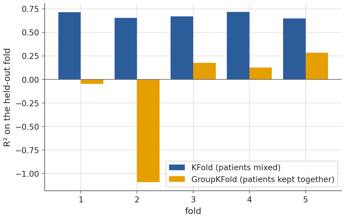
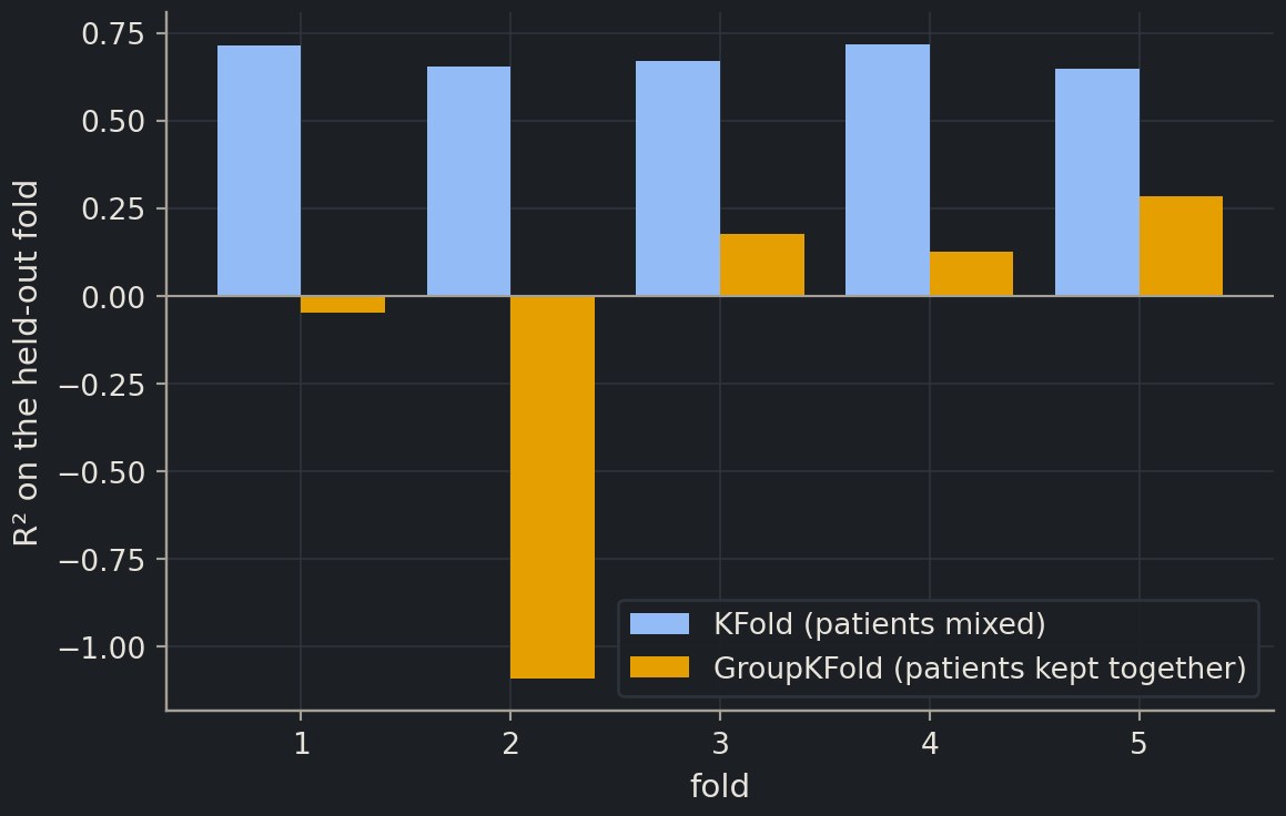
A plain KFold shuffles the 180 samples and puts some of every patient on both sides. GroupKFold takes a groups array and guarantees that all samples of a patient go to the same fold. Score a kNN regressor both ways.

from sklearn.model_selection import GroupKFold, KFold, cross_val_score

knn5 = KNeighborsRegressor(n_neighbors=5)
kfold = KFold(n_splits=5, shuffle=True, random_state=42)
group_kfold = GroupKFold(n_splits=5)

r2_kfold = cross_val_score(knn5, Xg, yg, cv=kfold)
r2_group = cross_val_score(knn5, Xg, yg, cv=group_kfold, groups=patient)
print(f"KFold      R² per fold: {np.round(r2_kfold, 2)}  mean {r2_kfold.mean():.2f}")
print(f"GroupKFold R² per fold: {np.round(r2_group, 2)}  mean {r2_group.mean():.2f}")

KFold      R² per fold: [0.72 0.65 0.67 0.72 0.65]  mean 0.68
GroupKFold R² per fold: [-0.05 -1.09  0.18  0.12  0.28]  mean -0.11

With the random split, kNN finds the patient’s own other samples by their fingerprint, copies their offset and reports \(R^2 \approx 0.7\). With the group split it has to predict a new patient from the signal alone, and the honest answer is that this model cannot: \(R^2\) is about zero. The first number is what the paper would have reported; the second is what the clinic would have observed.

import matplotlib.pyplot as plt

fig, ax = plt.subplots(figsize=(6, 3.8))
folds = np.arange(1, 6)
ax.bar(folds - 0.2, r2_kfold, width=0.4, label="KFold (patients mixed)")
ax.bar(folds + 0.2, r2_group, width=0.4, label="GroupKFold (patients kept together)")
ax.axhline(0, color="0.4", linewidth=0.8)
ax.set(xlabel="fold", ylabel="R² on the held-out fold", xticks=folds)
ax.legend()
plt.show()

Bar chart of R-squared per cross-validation fold for KFold and GroupKFold on the synthetic patient data. The five KFold bars are all around 0.65 to 0.7; the GroupKFold bars are scattered between minus 1.1 and 0.3, mostly near zero.

Biologist's corner

“Patient” stands for any unit that makes samples non-independent: the animal in a dose study, the litter, the cell line, the 96-well plate, the sequencing batch, the day the microscope was recalibrated. If the model can tell which unit a sample came from, a random split lets it exploit that. The rule is to split at the level at which you want to generalise: new patients, new plates, new batches. Part III applies the same rule to proteins, where “same group” means “similar sequence”: two proteins at 90% identity are the same patient in disguise.

GroupKFold is also the backbone of the scaffold split you meet in Part II: the group is the molecule’s core ring system, so the test set contains chemotypes the model never saw.

Preprocessing before splitting

Fit a StandardScaler on all of ESOL, then split, then model. Compare with the honest order.

Xtr, Xte, ytr, yte = train_test_split(Xe, ye, test_size=0.2, random_state=42)

leaky_scaler = StandardScaler().fit(Xe)                       # sees the test rows
leaky_knn = KNeighborsRegressor().fit(leaky_scaler.transform(Xtr), ytr)
honest_scaler = StandardScaler().fit(Xtr)
honest_knn = KNeighborsRegressor().fit(honest_scaler.transform(Xtr), ytr)

print(f"scaler fitted on everything: RMSE {root_mean_squared_error(yte, leaky_knn.predict(leaky_scaler.transform(Xte))):.4f}")
print(f"scaler fitted on train only: RMSE {root_mean_squared_error(yte, honest_knn.predict(honest_scaler.transform(Xte))):.4f}")

scaler fitted on everything: RMSE 0.9493
scaler fitted on train only: RMSE 0.9494

The difference is in the third decimal: the test rows nudge the means and standard deviations by a fraction of a percent. Scaling leaks little because it does not look at y. Preprocessing that does look at y is a different story. Here is a dataset of 200 samples with 1,000 features of pure noise and a target of pure noise. Pick the ten features most correlated with the target, using all the data, and then “evaluate” properly.

rng = np.random.default_rng(42)
X_noise = rng.normal(size=(200, 1000))
y_noise = rng.normal(size=200)


def top_correlated(X, y, k=10):
    corr = np.array([abs(np.corrcoef(X[:, j], y)[0, 1]) for j in range(X.shape[1])])
    return np.argsort(corr)[-k:]


from sklearn.linear_model import LinearRegression

chosen = top_correlated(X_noise, y_noise)                    # selected on ALL the data
Xtr, Xte, ytr, yte = train_test_split(X_noise[:, chosen], y_noise, test_size=0.2, random_state=42)
leaky_r2 = LinearRegression().fit(Xtr, ytr).score(Xte, yte)

Xtr, Xte, ytr, yte = train_test_split(X_noise, y_noise, test_size=0.2, random_state=42)
chosen = top_correlated(Xtr, ytr)                            # selected on the training rows
honest_r2 = LinearRegression().fit(Xtr[:, chosen], ytr).score(Xte[:, chosen], yte)
print(f"test R², features selected on all data:   {leaky_r2:.2f}")
print(f"test R², features selected on train only: {honest_r2:.2f}")

test R², features selected on all data:   0.29
test R², features selected on train only: -0.24

The leaky version reports \(R^2 \approx 0.29\) for predicting noise from noise. Among 1,000 random columns, some correlate with any target by chance; selecting them on the full table bakes the test rows’ chance correlations into the “model”, and the split afterwards cannot undo it. The honest version is negative, which is the correct answer. Gene-expression studies with thousands of genes and dozens of samples are exactly this shape, and this mistake has been made in print many times.

Maths corner

A test estimate is unbiased only if the test samples are independent of everything used to build the predictor. A scaler fitted on the full table makes the predictor a function of the test inputs \(x_{\text{test}}\) (through the estimated mean and variance), which breaks independence mildly. Selecting features by their correlation with \(y\) makes the predictor a function of the test labels: the selected set is chosen to maximise \(|\hat{\rho}(x_j, y)|\) over all rows, so the test residuals are small by construction, not by generalisation. The size of the bias grows with the number of candidates searched, which is why high-dimensional data (many features, few samples) is where this leak bites hardest.

Target leakage

The last route is a column that is recorded after, or because of, the outcome. A thought experiment: you predict whether a tumour is malignant from a hospital database, and one column is “chemotherapy started (yes/no)”. It is a near-perfect predictor and completely useless, because it was filled in after the diagnosis you are trying to predict. That is target leakage. Other examples: “days until the next appointment” when predicting readmission, a cell-viability readout when predicting toxicity, or, closer to home, the ESOL predicted log solubility column in our file, which is the output of a model that was fitted on the measured values. Using it as a feature would launder Delaney’s training labels into our features.

Target leakage never shows up in a cross-validation score, which looks wonderful. The only defence is to ask, for every column, “would this value exist, with this value, at the moment I want to make the prediction?” If not, drop it.

Saving a pipeline

A fitted pipeline is one Python object, so it can be saved as one file. scikit-learn uses joblib for this. Here the file goes to a temporary directory; in a project you would write it next to the data with a versioned name.

import tempfile

import joblib

with tempfile.TemporaryDirectory() as tmp:
    model_path = Path(tmp) / "penguin_ridge.joblib"
    joblib.dump(penguin_model, model_path)
    reloaded = joblib.load(model_path)
    same = np.allclose(reloaded.predict(Xp_test), penguin_model.predict(Xp_test))
    print(f"saved {model_path.stat().st_size / 1024:.1f} kB; predictions identical: {same}")

saved 4.0 kB; predictions identical: True

Saving the pipeline rather than the model alone is the point: the file contains the medians, the category lists and the scaling constants, so a colleague who loads it can feed it raw penguin rows and get the same predictions. A model saved without its preprocessing is a model nobody can use. Two caveats: a joblib file is only guaranteed to load with the same scikit-learn version, and like a pickle it executes code when loaded, so load only files you trust.

Tip

Reproducibility checklist

Seeds everywhere: random_state=42 in splits, models and searches; np.random.default_rng(42) for your own randomness.
Pinned versions: install from environment.yml or requirements.txt and run python scripts/check_env.py before you start; record its output.
One pipeline, not loose steps: every fitted preprocessing step lives inside the Pipeline you save.
Split once and store the indices: write X_test.index to a file so that every later experiment uses the same test molecules.
Record the git commit of the code that produced each result, and the dataset checksum (scripts/fetch_data.py prints it).
Never touch the test set twice: all choices come from cross-validation on the training set; the test set is evaluated once, at the end.
Log everything: hyperparameters, CV scores, test scores and the date, in a table you can rerun.

Discussion

A paper reports 94% accuracy for predicting antibiotic resistance from bacterial genomes, with 2,000 isolates collected from 40 hospitals and a random 80/20 split. Which of the four leaks is most likely, and what single change to the evaluation would you ask the authors to make?

Exercises

Exercise★☆☆

A pipeline for penguin species

Build a ColumnTransformer + LogisticRegression pipeline that predicts species from the three bill/flipper measurements and sex (which has missing values). Use median imputation for the numbers, most-frequent imputation and one-hot encoding for sex, a stratified 80/20 split with random_state=42, and report the test accuracy and the output feature names. Which step would fail if you removed the imputer for sex?

SolutionShow solution

Xs = penguins[numeric + ["sex"]]
ys = penguins["species"]
Xs_train, Xs_test, ys_train, ys_test = train_test_split(
    Xs, ys, test_size=0.2, stratify=ys, random_state=42
)
species_pre = ColumnTransformer(
    [
        ("num", make_pipeline(SimpleImputer(strategy="median"), StandardScaler()), numeric),
        ("sex", make_pipeline(SimpleImputer(strategy="most_frequent"),
                              OneHotEncoder(handle_unknown="ignore")), ["sex"]),
    ]
)
species_model = make_pipeline(species_pre, LogisticRegression(max_iter=1000)).fit(Xs_train, ys_train)
print(f"test accuracy: {species_model.score(Xs_test, ys_test):.3f}")
print(species_model[:-1].get_feature_names_out())

test accuracy: 1.000
['num__bill_length_mm' 'num__bill_depth_mm' 'num__flipper_length_mm'
 'sex__sex_female' 'sex__sex_male']

Nothing would actually fail without the sex imputer: OneHotEncoder treats NaN as a category of its own and adds a sex_nan column. That is a design choice, not a bug, and sometimes it is the right one (missingness can be informative). What would fail is removing the numeric imputer, because LogisticRegression raises an error on NaN inputs. Species is an easy target: the three measurements separate the species almost perfectly, so the accuracy is near 1.

Exercise★★☆

Rank the leaks

Five modelling set-ups, all with a random 80/20 split and a good-looking test score. Rank them from most to least severe leakage and say in one sentence why.

A. Predicting toxicity from 2,000 descriptors; the 50 descriptors most correlated with toxicity were chosen on the full dataset before splitting. B. Predicting protein function; the dataset contains many pairs of sequences at more than 95% identity. C. Predicting solubility; the features were standardised with a StandardScaler fitted on the full dataset. D. Predicting hospital readmission; one feature is the number of follow-up appointments booked after discharge. E. Predicting binding affinity; 30% of the compounds appear twice under different IDs with the same measurement.

SolutionShow solution

A defensible ranking, most severe first: D, A, E, B, C.

D (target leakage). The feature is recorded after the outcome and partly caused by it. No evaluation scheme can reveal this; the model is useless in deployment.
A (target-dependent preprocessing before the split). Selecting 50 of 2,000 features by correlation with y on all rows bakes the test labels into the feature set; on pure noise this produces \(R^2\) of 0.2–0.3, and with real signal it inflates the score by a similar margin.
E (exact duplicates). With 30% duplicated rows, roughly a third of the test set has an identical twin in training. For memorising models (kNN, trees) the score is badly inflated; for a rigid linear model less so, which is why it ranks below A.
B (near-duplicate groups). The same mechanism as E, but graded: 95% identity is “almost the same sample”. Severity depends on how many such pairs exist; the fix is a group split by sequence cluster.
C (scaling before the split). Conceptually wrong, numerically negligible: the leak is a few decimals of a mean and a standard deviation. Fix it anyway, because the pipeline habit is what prevents A.

Reasonable people may swap A and E depending on the model; the important boundary is that D and A involve the labels, while B, C and E involve only the inputs.

Exercise★★★

A crude scaffold split for ESOL

Scaffold splits need RDKit (Part II). As a stand-in, bin the ESOL molecules into ten groups by molecular weight with pd.qcut(esol["Molecular Weight"], 10, labels=False) and use those bins as groups in a GroupKFold. Compare the cross-validated RMSE of the scaled kNN regressor under KFold(5, shuffle=True, random_state=42) and under GroupKFold(5). Which is larger, and why is this a (very) rough proxy for predicting new chemistry?

SolutionShow solution

mw_bins = pd.qcut(esol["Molecular Weight"], 10, labels=False)
rmse_random = -cross_val_score(knn_reg, Xe, ye, cv=kfold, scoring="neg_root_mean_squared_error")
rmse_group = -cross_val_score(knn_reg, Xe, ye, cv=group_kfold, groups=mw_bins,
                              scoring="neg_root_mean_squared_error")
print(f"random folds:            RMSE {rmse_random.mean():.3f} logS")
print(f"molecular-weight groups: RMSE {rmse_group.mean():.3f} logS")

random folds:            RMSE 0.925 logS
molecular-weight groups: RMSE 1.119 logS

The grouped RMSE is about 0.2 log units higher. Under GroupKFold each held-out fold contains a range of weights the model never saw, so kNN must extrapolate to molecules unlike its neighbours instead of interpolating between them. That is the situation a real project faces: the next series of compounds is heavier, or has a new ring system, and a random split never asks the model that question. Molecular weight is a crude proxy because two molecules of equal weight can be chemically unrelated; a scaffold split groups by the ring framework, which is closer to what a chemist means by “new chemistry”. Expect the gap to be larger still there.

Where this is going

Everything you evaluate from now on goes through a pipeline, and every split is chosen by asking “what will the next sample look like?” In Part II the groups become Murcko scaffolds and the pipeline’s first step becomes a fingerprint computed with RDKit; in Part III the groups become sequence-identity clusters and the first step an embedding of the protein sequence. The leakage catalogue stays the same, and so does the fix. Lab 2 puts the whole chapter together on the solubility problem, from baseline to saved pipeline; the chapter checkpoint lets you test yourself first.

Key points

Scale features for kNN, logistic regression, ridge and lasso; fit the scaler on the training data only.
A Pipeline bundles preprocessing and model into one estimator: fit learns everything from the training set, predict applies it unchanged to new data.
ColumnTransformer sends numeric columns through imputation and scaling and categorical columns through one-hot encoding; get_feature_names_out() tells you what came out.
Leakage is any way information about the test set reaches the model before evaluation. The test score then measures memory, not generalisation.
Duplicates, repeated patients or batches, preprocessing fitted on all data and after-the-fact columns are the four leaks to check for in every scientific dataset.
GroupKFold keeps every sample of a group on one side of the split; scaffold and sequence-identity splits are the same idea for molecules and proteins.
Save the whole pipeline with joblib.dump, fix every seed, pin versions and never touch the test set twice.

	transformers transformers: list of tuples List of (name, transformer, columns) tuples specifying the transformer objects to be applied to subsets of the data. name : str Like in Pipeline and FeatureUnion, this allows the transformer and its parameters to be set using ``set_params`` and searched in grid search. transformer : {'drop', 'passthrough'} or estimator Estimator must support :term:`fit` and :term:`transform`. Special-cased strings 'drop' and 'passthrough' are accepted as well, to indicate to drop the columns or to pass them through untransformed, respectively. columns : str, array-like of str, int, array-like of int, array-like of bool, slice or callable Indexes the data on its second axis. Integers are interpreted as positional columns, while strings can reference DataFrame columns by name. A scalar string or int should be used where ``transformer`` expects X to be a 1d array-like (vector), otherwise a 2d array will be passed to the transformer. A callable is passed the input data `X` and can return any of the above. To select multiple columns by name or dtype, you can use :obj:`make_column_selector`.	[('num', ...), ('cat', ...)]
	remainder remainder: {'drop', 'passthrough'} or estimator, default='drop' By default, only the specified columns in `transformers` are transformed and combined in the output, and the non-specified columns are dropped. (default of ``'drop'``). By specifying ``remainder='passthrough'``, all remaining columns that were not specified in `transformers`, but present in the data passed to `fit` will be automatically passed through. This subset of columns is concatenated with the output of the transformers. For dataframes, extra columns not seen during `fit` will be excluded from the output of `transform`. By setting ``remainder`` to be an estimator, the remaining non-specified columns will use the ``remainder`` estimator. The estimator must support :term:`fit` and :term:`transform`. Note that using this feature requires that the DataFrame columns input at :term:`fit` and :term:`transform` have identical order.	'drop'
	sparse_threshold sparse_threshold: float, default=0.3 If the output of the different transformers contains sparse matrices, these will be stacked as a sparse matrix if the overall density is lower than this value. Use ``sparse_threshold=0`` to always return dense. When the transformed output consists of all dense data, the stacked result will be dense, and this keyword will be ignored.	0.3
	n_jobs n_jobs: int, default=None Number of jobs to run in parallel. ``None`` means 1 unless in a :obj:`joblib.parallel_backend` context. ``-1`` means using all processors. See :term:`Glossary <n_jobs>` for more details.	None
	transformer_weights transformer_weights: dict, default=None Multiplicative weights for features per transformer. The output of the transformer is multiplied by these weights. Keys are transformer names, values the weights.	None
	verbose verbose: bool, default=False If True, the time elapsed while fitting each transformer will be printed as it is completed.	False
	verbose_feature_names_out verbose_feature_names_out: bool, str or Callable[[str, str], str], default=True - If True, :meth:`ColumnTransformer.get_feature_names_out` will prefix all feature names with the name of the transformer that generated that feature. It is equivalent to setting `verbose_feature_names_out="{transformer_name}__{feature_name}"`. - If False, :meth:`ColumnTransformer.get_feature_names_out` will not prefix any feature names and will error if feature names are not unique. - If ``Callable[[str, str], str]``, :meth:`ColumnTransformer.get_feature_names_out` will rename all the features using the name of the transformer. The first argument of the callable is the transformer name and the second argument is the feature name. The returned string will be the new feature name. - If ``str``, it must be a string ready for formatting. The given string will be formatted using two field names: ``transformer_name`` and ``feature_name``. e.g. ``"{feature_name}__{transformer_name}"``. See :meth:`str.format` method from the standard library for more info. .. versionadded:: 1.0 .. versionchanged:: 1.6 `verbose_feature_names_out` can be a callable or a string to be formatted.	True

	strategy strategy: str or Callable, default='mean' The imputation strategy. - If "mean", then replace missing values using the mean along each column. Can only be used with numeric data. - If "median", then replace missing values using the median along each column. Can only be used with numeric data. - If "most_frequent", then replace missing using the most frequent value along each column. Can be used with strings or numeric data. If there is more than one such value, only the smallest is returned. - If "constant", then replace missing values with fill_value. Can be used with strings or numeric data. - If an instance of Callable, then replace missing values using the scalar statistic returned by running the callable over a dense 1d array containing non-missing values of each column. .. versionadded:: 0.20 strategy="constant" for fixed value imputation. .. versionadded:: 1.5 strategy=callable for custom value imputation.	'median'
	missing_values missing_values: int, float, str, np.nan, None or pandas.NA, default=np.nan The placeholder for the missing values. All occurrences of `missing_values` will be imputed. For pandas' dataframes with nullable integer dtypes with missing values, `missing_values` can be set to either `np.nan` or `pd.NA`.	nan
	fill_value fill_value: str or numerical value, default=None When strategy == "constant", `fill_value` is used to replace all occurrences of missing_values. For string or object data types, `fill_value` must be a string. If `None`, `fill_value` will be 0 when imputing numerical data and "missing_value" for strings or object data types.	None
	copy copy: bool, default=True If True, a copy of X will be created. If False, imputation will be done in-place whenever possible. Note that, in the following cases, a new copy will always be made, even if `copy=False`: - If `X` is not an array of floating values; - If `X` is encoded as a CSR matrix; - If `add_indicator=True`.	True
	add_indicator add_indicator: bool, default=False If True, a :class:`MissingIndicator` transform will stack onto output of the imputer's transform. This allows a predictive estimator to account for missingness despite imputation. If a feature has no missing values at fit/train time, the feature won't appear on the missing indicator even if there are missing values at transform/test time.	False
	keep_empty_features keep_empty_features: bool, default=False If True, features that consist exclusively of missing values when `fit` is called are returned in results when `transform` is called. The imputed value is always `0` except when `strategy="constant"` in which case `fill_value` will be used instead. .. versionadded:: 1.2	False

	strategy strategy: str or Callable, default='mean' The imputation strategy. - If "mean", then replace missing values using the mean along each column. Can only be used with numeric data. - If "median", then replace missing values using the median along each column. Can only be used with numeric data. - If "most_frequent", then replace missing using the most frequent value along each column. Can be used with strings or numeric data. If there is more than one such value, only the smallest is returned. - If "constant", then replace missing values with fill_value. Can be used with strings or numeric data. - If an instance of Callable, then replace missing values using the scalar statistic returned by running the callable over a dense 1d array containing non-missing values of each column. .. versionadded:: 0.20 strategy="constant" for fixed value imputation. .. versionadded:: 1.5 strategy=callable for custom value imputation.	'most_frequent'
	missing_values missing_values: int, float, str, np.nan, None or pandas.NA, default=np.nan The placeholder for the missing values. All occurrences of `missing_values` will be imputed. For pandas' dataframes with nullable integer dtypes with missing values, `missing_values` can be set to either `np.nan` or `pd.NA`.	nan
	fill_value fill_value: str or numerical value, default=None When strategy == "constant", `fill_value` is used to replace all occurrences of missing_values. For string or object data types, `fill_value` must be a string. If `None`, `fill_value` will be 0 when imputing numerical data and "missing_value" for strings or object data types.	None
	copy copy: bool, default=True If True, a copy of X will be created. If False, imputation will be done in-place whenever possible. Note that, in the following cases, a new copy will always be made, even if `copy=False`: - If `X` is not an array of floating values; - If `X` is encoded as a CSR matrix; - If `add_indicator=True`.	True
	add_indicator add_indicator: bool, default=False If True, a :class:`MissingIndicator` transform will stack onto output of the imputer's transform. This allows a predictive estimator to account for missingness despite imputation. If a feature has no missing values at fit/train time, the feature won't appear on the missing indicator even if there are missing values at transform/test time.	False
	keep_empty_features keep_empty_features: bool, default=False If True, features that consist exclusively of missing values when `fit` is called are returned in results when `transform` is called. The imputed value is always `0` except when `strategy="constant"` in which case `fill_value` will be used instead. .. versionadded:: 1.2	False

	handle_unknown handle_unknown: {'error', 'ignore', 'infrequent_if_exist', 'warn'}, default='error' Specifies the way unknown categories are handled during :meth:`transform`. - 'error' : Raise an error if an unknown category is present during transform. - 'ignore' : When an unknown category is encountered during transform, the resulting one-hot encoded columns for this feature will be all zeros. In the inverse transform, an unknown category will be denoted as None. - 'infrequent_if_exist' : When an unknown category is encountered during transform, the resulting one-hot encoded columns for this feature will map to the infrequent category if it exists. The infrequent category will be mapped to the last position in the encoding. During inverse transform, an unknown category will be mapped to the category denoted `'infrequent'` if it exists. If the `'infrequent'` category does not exist, then :meth:`transform` and :meth:`inverse_transform` will handle an unknown category as with `handle_unknown='ignore'`. Infrequent categories exist based on `min_frequency` and `max_categories`. Read more in the :ref:`User Guide <encoder_infrequent_categories>`. - 'warn' : When an unknown category is encountered during transform a warning is issued, and the encoding then proceeds as described for `handle_unknown="infrequent_if_exist"`. .. versionchanged:: 1.1 `'infrequent_if_exist'` was added to automatically handle unknown categories and infrequent categories. .. versionadded:: 1.6 The option `"warn"` was added in 1.6.	'ignore'
	categories categories: 'auto' or a list of array-like, default='auto' Categories (unique values) per feature: - 'auto' : Determine categories automatically from the training data. - list : ``categories[i]`` holds the categories expected in the ith column. The passed categories should not mix strings and numeric values within a single feature, and should be sorted in case of numeric values. The used categories can be found in the ``categories_`` attribute. .. versionadded:: 0.20	'auto'
	drop drop: {'first', 'if_binary'} or an array-like of shape (n_features,), default=None Specifies a methodology to use to drop one of the categories per feature. This is useful in situations where perfectly collinear features cause problems, such as when feeding the resulting data into an unregularized linear regression model. However, dropping one category breaks the symmetry of the original representation and can therefore induce a bias in downstream models, for instance for penalized linear classification or regression models. - None : retain all features (the default). - 'first' : drop the first category in each feature. If only one category is present, the feature will be dropped entirely. - 'if_binary' : drop the first category in each feature with two categories. Features with 1 or more than 2 categories are left intact. - array : ``drop[i]`` is the category in feature ``X[:, i]`` that should be dropped. When `max_categories` or `min_frequency` is configured to group infrequent categories, the dropping behavior is handled after the grouping. .. versionadded:: 0.21 The parameter `drop` was added in 0.21. .. versionchanged:: 0.23 The option `drop='if_binary'` was added in 0.23. .. versionchanged:: 1.1 Support for dropping infrequent categories.	None
	sparse_output sparse_output: bool, default=True When ``True``, it returns a SciPy sparse matrix/array in "Compressed Sparse Row" (CSR) format. .. versionadded:: 1.2 `sparse` was renamed to `sparse_output`	True
	dtype dtype: number type, default=np.float64 Desired dtype of output.	<class 'numpy.float64'>
	min_frequency min_frequency: int or float, default=None Specifies the minimum frequency below which a category will be considered infrequent. - If `int`, categories with a smaller cardinality will be considered infrequent. - If `float`, categories with a smaller cardinality than `min_frequency * n_samples` will be considered infrequent. .. versionadded:: 1.1 Read more in the :ref:`User Guide <encoder_infrequent_categories>`.	None
	max_categories max_categories: int, default=None Specifies an upper limit to the number of output features for each input feature when considering infrequent categories. If there are infrequent categories, `max_categories` includes the category representing the infrequent categories along with the frequent categories. If `None`, there is no limit to the number of output features. .. versionadded:: 1.1 Read more in the :ref:`User Guide <encoder_infrequent_categories>`.	None
	feature_name_combiner feature_name_combiner: "concat" or callable, default="concat" Callable with signature `def callable(input_feature, category)` that returns a string. This is used to create feature names to be returned by :meth:`get_feature_names_out`. `"concat"` concatenates encoded feature name and category with `feature + "_" + str(category)`.E.g. feature X with values 1, 6, 7 create feature names `X_1, X_6, X_7`. .. versionadded:: 1.3	'concat'