Lab 1 solutions: Guided EDA of the breast cancer dataset

Lab 1: Guided EDA of the breast cancer Wisconsin dataset

In this lab you run the exploratory-data-analysis checklist from episode 1.5 on a new dataset, without a tutor typing ahead of you. The data are 569 breast tumours imaged by fine-needle aspiration; for each tumour, 30 numbers describe the cell nuclei in the image, and a pathologist’s diagnosis (malignant or benign) is the label. Chapter 2 uses this same table to train a classifier, so the picture you build here is one you will need again.

Goals

• Inspect a new table systematically: shape, types, missing values, class balance and summary statistics.
• Compare the distributions of several features between two classes with histograms, KDEs and box plots.
• Read a correlation heatmap and a pairplot and say which features are redundant and which separate the classes.
• Rank features by how well they separate the classes, and write a short, honest summary of what you found.

How to work

• Run the cells from top to bottom. Each task builds on the previous one.
• Cells that start with # TODO are yours to write. The comment line states the task.
• Cells marked ✅ are checks: they tell you whether you are on track. If one fails, read the message and fix the cell above it.
• You will not be asked to change anything that is not marked TODO.

# Setup: works locally and on Google Colab. Installs only what is missing.
import importlib.util

try:
    import google.colab  # noqa: F401

    IN_COLAB = True
except ImportError:
    IN_COLAB = False

REQUIRED = {"numpy": "numpy", "pandas": "pandas", "matplotlib": "matplotlib", "seaborn": "seaborn", "sklearn": "scikit-learn"}
missing = [pkg for mod, pkg in REQUIRED.items() if importlib.util.find_spec(mod) is None]
if IN_COLAB and missing:
    %pip install -q {" ".join(missing)}

import numpy as np
import pandas as pd
import matplotlib.pyplot as plt
import seaborn as sns

# Use the same class order and colours in every figure.
diagnosis_order = ["malignant", "benign"]
diagnosis_palette = dict(zip(diagnosis_order, sns.color_palette("colorblind")[:2]))

print("running on Colab" if IN_COLAB else "running locally", "| missing packages:", missing or "none")

running locally | missing packages: none

The data

This dataset ships with scikit-learn, so there is nothing to download: load_breast_cancer(as_frame=True) returns a pandas DataFrame with the 30 features and an integer target column (0 = malignant, 1 = benign). We add a readable diagnosis column so that plots label themselves.

from sklearn.datasets import load_breast_cancer

bc = load_breast_cancer(as_frame=True)
df = bc.frame.assign(diagnosis=bc.frame["target"].map({0: "malignant", 1: "benign"}))
print(bc.target_names)  # index 0 -> malignant, index 1 -> benign
df.sample(5, random_state=42)

['malignant' 'benign']

index	mean radius	mean texture	mean perimeter	mean area	mean smoothness	mean compactness	mean concavity	mean concave points	mean symmetry	mean fractal dimension	...	worst perimeter	worst area	worst smoothness	worst compactness	worst concavity	worst concave points	worst symmetry	worst fractal dimension	target	diagnosis
204	12.47	18.60	81.09	481.9	0.09965	0.1058	0.08005	0.03821	0.1925	0.06373	...	96.05	677.9	0.1426	0.2378	0.2671	0.10150	0.3014	0.08750	1	benign
70	18.94	21.31	123.60	1130.0	0.09009	0.1029	0.10800	0.07951	0.1582	0.05461	...	165.90	1866.0	0.1193	0.2336	0.2687	0.17890	0.2551	0.06589	0	malignant
131	15.46	19.48	101.70	748.9	0.10920	0.1223	0.14660	0.08087	0.1931	0.05796	...	124.90	1156.0	0.1546	0.2394	0.3791	0.15140	0.2837	0.08019	0	malignant
431	12.40	17.68	81.47	467.8	0.10540	0.1316	0.07741	0.02799	0.1811	0.07102	...	89.61	515.8	0.1450	0.2629	0.2403	0.07370	0.2556	0.09359	1	benign
540	11.54	14.44	74.65	402.9	0.09984	0.1120	0.06737	0.02594	0.1818	0.06782	...	78.78	457.8	0.1345	0.2118	0.1797	0.06918	0.2329	0.08134	1	benign

5 rows × 32 columns

Loading the course CSVs elsewhere. Other labs read files from the course’s data/ folder (for example the penguins). On your own machine those files sit next to the notebook or at the repository root; on Colab they do not exist, so the helper below tries the local paths first and then falls back to the raw file on GitHub. You do not need it for this lab, but run it once so that you recognise the pattern when it appears in Lab 2.

from pathlib import Path


def load_course_csv(name: str) -> pd.DataFrame:
    """Read a course CSV from the first location that exists: next to the notebook, at the repo root, or GitHub."""
    candidates = [
        Path("data") / name,
        Path("../../../data") / name,
        f"https://raw.githubusercontent.com/Awguhst/MolModels/main/data/{name}",
    ]
    for candidate in candidates:
        if isinstance(candidate, str) or candidate.exists():
            return pd.read_csv(candidate)
    raise FileNotFoundError(name)


# Example (not needed below): penguins = load_course_csv("penguins.csv")
print("helper defined; first candidate path:", Path("data") / "penguins.csv")

helper defined; first candidate path: data/penguins.csv

Task 1: shape, types and missing values

Start exactly as in episode 1.5: how big is the table, what type is each column, and is anything missing? Store the number of missing values (over the whole table) in a variable called n_missing.

# Task 1: print df.shape, show df.dtypes, and compute n_missing = total number of missing values in df
print(df.shape)
print(df.dtypes.value_counts())
n_missing = int(df.isna().sum().sum())
print("missing values:", n_missing)

(569, 32)
float64    30
int64       1
str         1
Name: count, dtype: int64
missing values: 0

assert df.shape == (569, 32), "expected 569 rows and 32 columns (30 features + target + diagnosis)"
assert n_missing == 0, "this dataset has no missing values; check df.isna().sum().sum()"
print("✅ Task 1: 569 rows, 32 columns, no missing values")

✅ Task 1: 569 rows, 32 columns, no missing values

Task 2: class balance

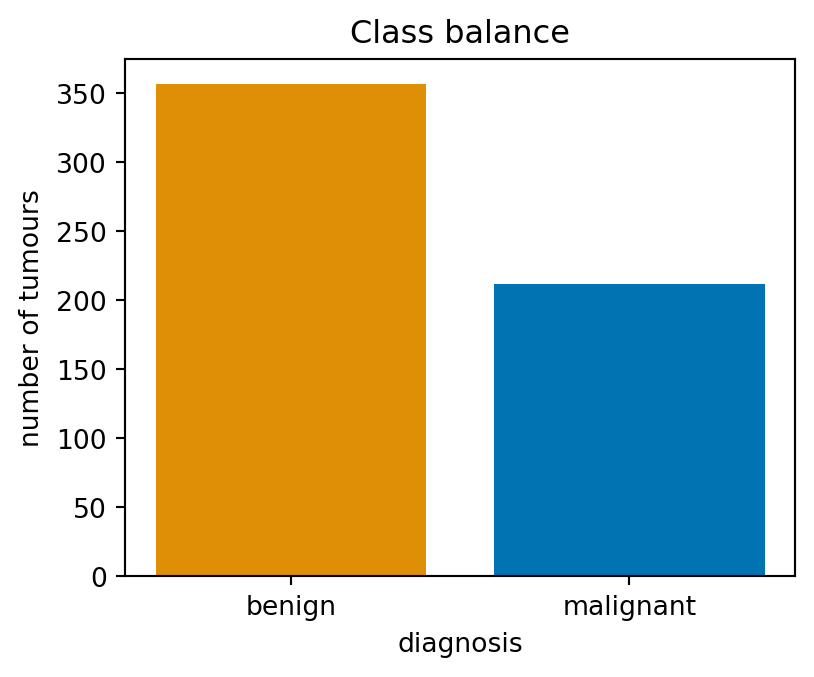
How many tumours of each class are there? Count them with value_counts() and store the result in counts, then draw a bar chart of the counts with the object-oriented matplotlib API (fig, ax = plt.subplots(); ax.bar(...)). Label the y axis. Use diagnosis_palette[label] to give each diagnosis the same colour as in the later plots.

# Task 2: counts = df["diagnosis"].value_counts(); then a bar chart of counts with labelled axes
counts = df["diagnosis"].value_counts()
print(counts)

fig, ax = plt.subplots(figsize=(4.5, 3.5))
ax.bar(counts.index, counts.values, color=[diagnosis_palette[label] for label in counts.index])
ax.set(xlabel="diagnosis", ylabel="number of tumours", title="Class balance")
plt.show()

diagnosis
benign       357
malignant    212
Name: count, dtype: int64

assert counts["benign"] == 357 and counts["malignant"] == 212, "expected 357 benign and 212 malignant"
print(f"✅ Task 2: {counts['malignant']} malignant, {counts['benign']} benign ({counts['benign'] / len(df):.0%} benign)")

✅ Task 2: 212 malignant, 357 benign (63% benign)

About 63% of the tumours are benign. Remember this number: in Chapter 2 a classifier that always says “benign” will score 63% accuracy while missing every malignant case, which is why accuracy alone is never enough.

Task 3: summary statistics

The 30 features come in three groups of ten: the mean ... of each nucleus measurement over the image, the ... error (standard error) and the worst ... (mean of the three largest values). Build a list mean_features of the ten column names that start with "mean ", then show describe() for those columns, transposed so that one row is one feature.

# Task 3: mean_features = the ten column names starting with "mean "; show df[mean_features].describe().T
mean_features = [c for c in df.columns if c.startswith("mean ")]
df[mean_features].describe().T.round(3)

index	count	mean	std	min	25%	50%	75%	max
mean radius	569.0	14.127	3.524	6.981	11.700	13.370	15.780	28.110
mean texture	569.0	19.290	4.301	9.710	16.170	18.840	21.800	39.280
mean perimeter	569.0	91.969	24.299	43.790	75.170	86.240	104.100	188.500
mean area	569.0	654.889	351.914	143.500	420.300	551.100	782.700	2501.000
mean smoothness	569.0	0.096	0.014	0.053	0.086	0.096	0.105	0.163
mean compactness	569.0	0.104	0.053	0.019	0.065	0.093	0.130	0.345
mean concavity	569.0	0.089	0.080	0.000	0.030	0.062	0.131	0.427
mean concave points	569.0	0.049	0.039	0.000	0.020	0.034	0.074	0.201
mean symmetry	569.0	0.181	0.027	0.106	0.162	0.179	0.196	0.304
mean fractal dimension	569.0	0.063	0.007	0.050	0.058	0.062	0.066	0.097

assert len(mean_features) == 10, f"expected 10 'mean' features, got {len(mean_features)}"
assert all(c.startswith("mean ") for c in mean_features), "every name should start with 'mean '"
print("✅ Task 3:", ", ".join(c.replace("mean ", "") for c in mean_features))

✅ Task 3: radius, texture, perimeter, area, smoothness, compactness, concavity, concave points, symmetry, fractal dimension

Look at the max column against the mean column. mean area runs from 144 to 2501, while mean smoothness runs from 0.05 to 0.16: the features live on wildly different scales. That will matter for every model in Chapter 2 that measures distances, and it is why we do not put raw features of different units on one axis.

Task 4: distributions by diagnosis

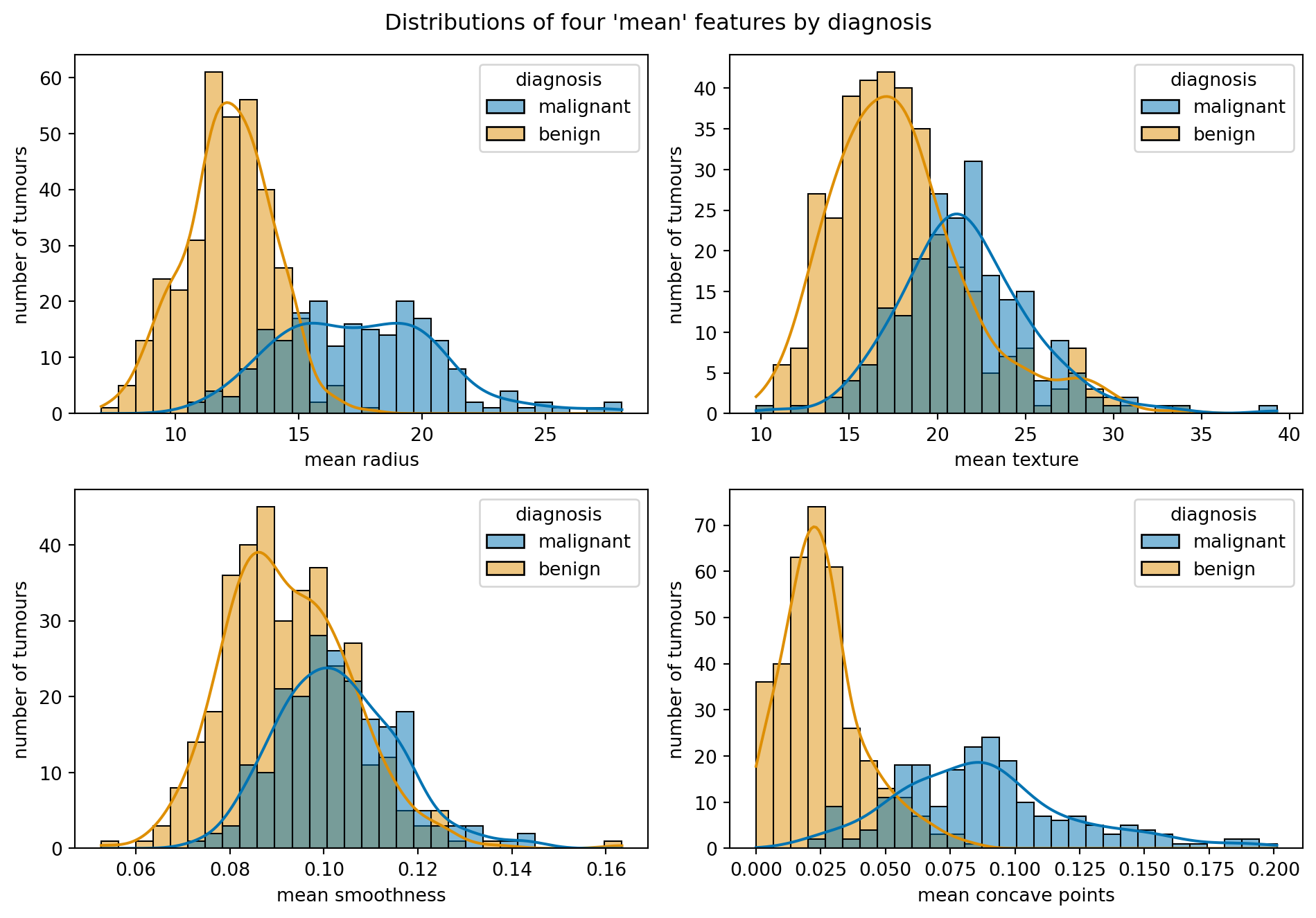
Draw a 2 × 2 grid of histograms with KDE curves for mean radius, mean texture, mean smoothness and mean concave points, each split by diagnosis (hue). Use sns.histplot(..., kde=True, ax=ax) and loop over axes.flat. Which of the four features separates the classes most clearly by eye? Use hue_order=diagnosis_order and palette=diagnosis_palette for consistent class colours.

# Task 4: 2x2 grid of sns.histplot(..., hue="diagnosis", kde=True) for the four features below
four = ["mean radius", "mean texture", "mean smoothness", "mean concave points"]

fig, axes = plt.subplots(2, 2, figsize=(10, 7))
for ax, col in zip(axes.flat, four):
    sns.histplot(data=df, x=col, hue="diagnosis", hue_order=diagnosis_order,
                 palette=diagnosis_palette, kde=True, bins=30, ax=ax)
    ax.set(ylabel="number of tumours")
fig.suptitle("Distributions of four 'mean' features by diagnosis")
fig.tight_layout()
plt.show()

assert set(four) <= set(df.columns), "one of the four feature names is misspelt"
print("✅ Task 4: four histograms drawn")

✅ Task 4: four histograms drawn

mean concave points and mean radius separate the classes well: the malignant distribution sits clearly to the right, with limited overlap. mean smoothness and especially mean texture overlap heavily. Keep this impression; Task 8 puts a number on it.

Task 5: box plots

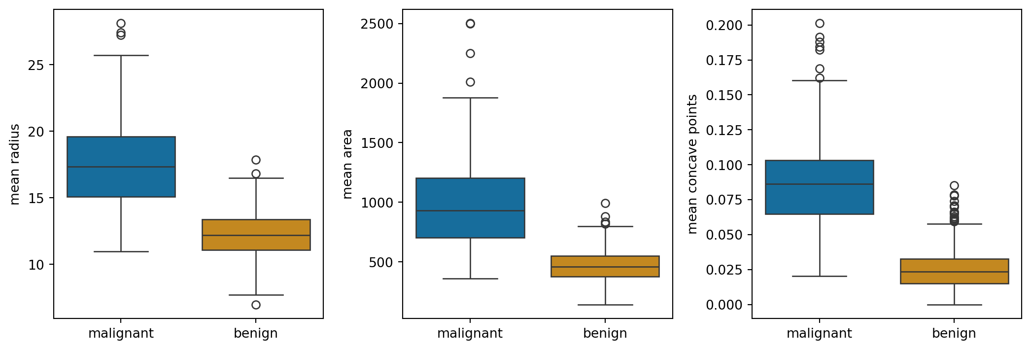
Box plots show the same comparison more compactly. Draw a 1 × 3 row of box plots of mean radius, mean area and mean concave points by diagnosis (sns.boxplot(data=df, x="diagnosis", y=..., hue="diagnosis", legend=False, ax=ax)). Then compute medians: the median of mean radius per diagnosis, via groupby. Keep order=diagnosis_order, hue_order=diagnosis_order and palette=diagnosis_palette.

# Task 5: three box plots by diagnosis, then medians = df.groupby("diagnosis")["mean radius"].median()
fig, axes = plt.subplots(1, 3, figsize=(11, 3.8))
for ax, col in zip(axes, ["mean radius", "mean area", "mean concave points"]):
    sns.boxplot(data=df, x="diagnosis", y=col, hue="diagnosis", order=diagnosis_order,
                hue_order=diagnosis_order, palette=diagnosis_palette, legend=False, ax=ax)
    ax.set(xlabel="")
fig.tight_layout()
plt.show()

medians = df.groupby("diagnosis")["mean radius"].median()
medians

diagnosis
benign       12.200
malignant    17.325
Name: mean radius, dtype: float64

assert medians["malignant"] > medians["benign"], "malignant tumours should have the larger median radius"
assert abs(medians["malignant"] - 17.3) < 0.2 and abs(medians["benign"] - 12.2) < 0.2, "unexpected medians; check the groupby"
print(f"✅ Task 5: median mean radius is {medians['malignant']:.1f} (malignant) vs {medians['benign']:.1f} (benign)")

✅ Task 5: median mean radius is 17.3 (malignant) vs 12.2 (benign)

Malignant nuclei are larger (median radius about 17 versus 12) and far more irregular (concave points). Note the outliers above the benign boxes: a few benign tumours have nuclei as large as a typical malignant one, which is where any classifier will make mistakes.

Task 6: correlation heatmap

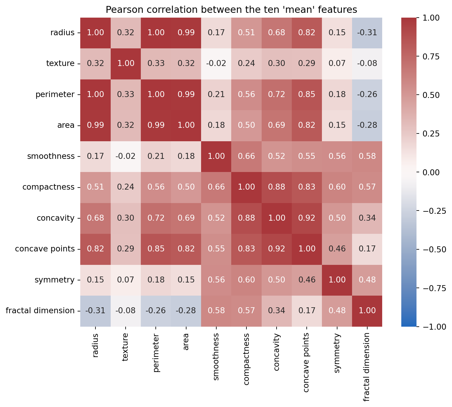
Compute the Pearson correlation matrix of the ten mean_features and store it in corr. Draw it with sns.heatmap(corr, annot=True, fmt=".2f", vmin=-1, vmax=1, cmap="vlag"). Shorten the tick labels by stripping the "mean " prefix (corr.rename(columns=..., index=...) or set the tick labels on the axes). Which pairs of features are nearly interchangeable?

# Task 6: corr = correlation matrix of df[mean_features]; heatmap with annot=True, fmt=".2f", vmin=-1, vmax=1
corr = df[mean_features].corr()
short = {c: c.replace("mean ", "") for c in mean_features}

fig, ax = plt.subplots(figsize=(8.5, 7))
sns.heatmap(corr.rename(columns=short, index=short), annot=True, fmt=".2f", vmin=-1, vmax=1, cmap="vlag", ax=ax)
ax.set(title="Pearson correlation between the ten 'mean' features")
plt.show()

assert corr.shape == (10, 10), "corr should be a 10 x 10 matrix of the 'mean' features"
assert abs(corr.loc["mean radius", "mean perimeter"] - 1.0) < 0.01, "radius and perimeter should correlate almost perfectly"
print(f"✅ Task 6: radius–perimeter r = {corr.loc['mean radius', 'mean perimeter']:.3f}, radius–area r = {corr.loc['mean radius', 'mean area']:.3f}")

✅ Task 6: radius–perimeter r = 0.998, radius–area r = 0.987

Radius, perimeter and area are three measurements of one thing, size, and correlate at approximately 0.99 or above. Compactness, concavity and concave points form a second block (0.8 to 0.9). These strong correlations show substantial redundancy, although correlation alone does not determine how many features a predictive model needs.

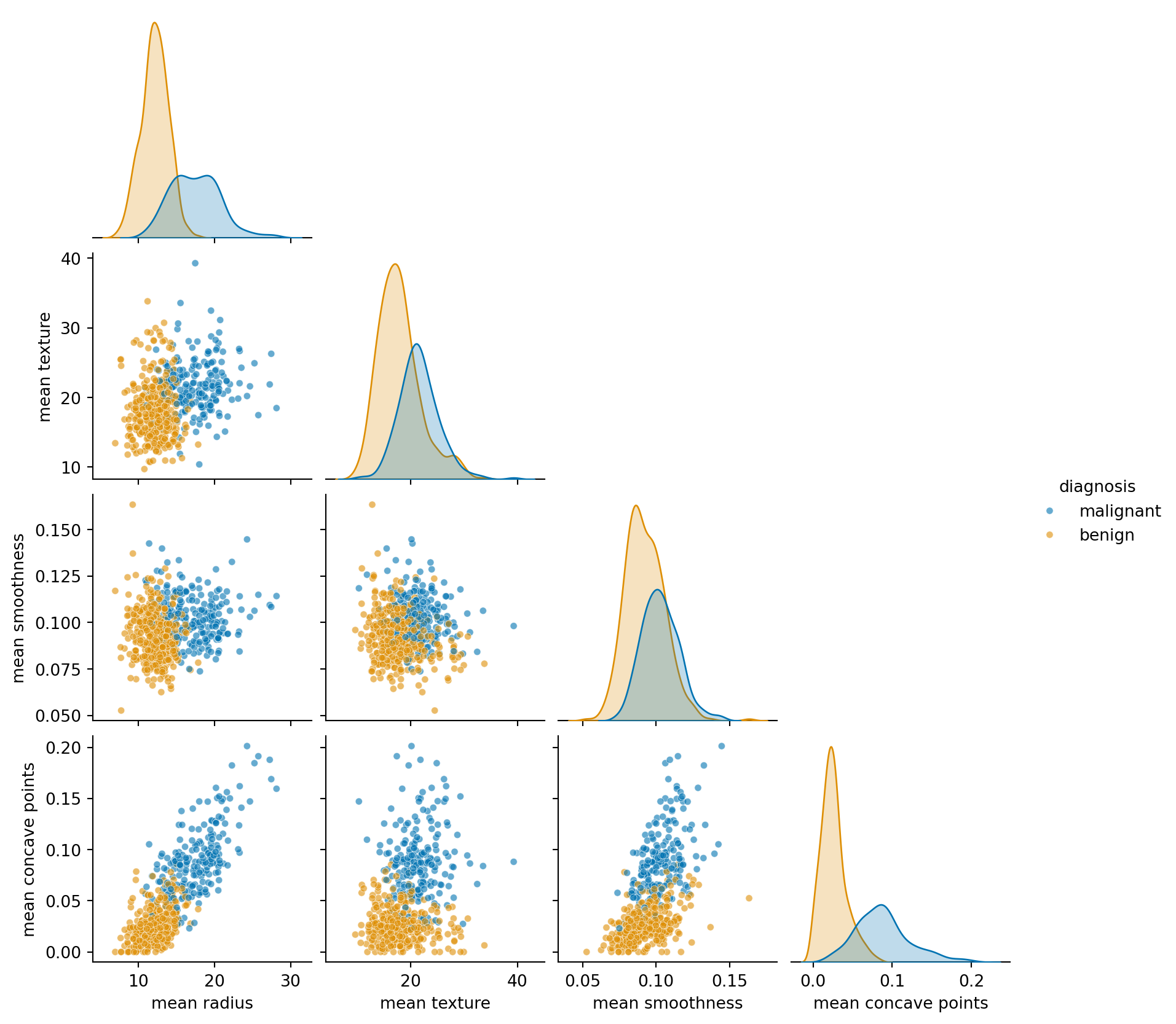
Task 7: pairplot

Draw a pairplot of mean radius, mean texture, mean smoothness and mean concave points, coloured by diagnosis, with corner=True. (sns.pairplot is a figure-level function: do not call plt.subplots() first.) Which pair of features separates the classes best? Reuse hue_order=diagnosis_order and palette=diagnosis_palette here too.

# Task 7: sns.pairplot of df[four + ["diagnosis"]], hue="diagnosis", corner=True
sns.pairplot(df[four + ["diagnosis"]], hue="diagnosis", hue_order=diagnosis_order,
             palette=diagnosis_palette, corner=True, height=2.2, plot_kws={"alpha": 0.6, "s": 18})
plt.show()

print("✅ Task 7: pairplot drawn (if the previous cell shows a triangular grid of 10 panels)")

✅ Task 7: pairplot drawn (if the previous cell shows a triangular grid of 10 panels)

mean radius against mean concave points gives the cleanest split: the benign tumours bunch in the bottom-left corner (small, smooth nuclei) and the malignant ones spread up and to the right. Combining two features separates more than either alone, which is the whole idea behind the classifiers in Chapter 2.

Task 8: which features separate the classes best?

Eyeballing histograms does not scale to 30 features. A simple score for how well a feature separates two groups is the standardised mean difference: the difference between the group means divided by the pooled standard deviation,

\[d = \frac{|\bar{x}_{\text{malignant}} - \bar{x}_{\text{benign}}|}{\sqrt{(s^2_{\text{malignant}} + s^2_{\text{benign}}) / 2}} .\]

A \(d\) of 0 means the groups have the same mean; a \(d\) above 2 means their means are more than two within-group standard deviations apart on this scale. It does not by itself guarantee little overlap. Compute \(d\) for all 30 numeric features (every column except target and diagnosis), store the result as a Series separation sorted from largest to smallest, and print the top five.

# Task 8: separation = standardised mean difference of every feature between the two classes, sorted descending
features = [c for c in df.columns if c not in ("target", "diagnosis")]
grouped = df.groupby("diagnosis")[features]
means, stds = grouped.mean(), grouped.std()
pooled = np.sqrt((stds.loc["malignant"] ** 2 + stds.loc["benign"] ** 2) / 2)
separation = ((means.loc["malignant"] - means.loc["benign"]).abs() / pooled).sort_values(ascending=False)
separation.head(5).round(2)

worst concave points    2.60
worst perimeter         2.37
mean concave points     2.33
worst radius            2.32
mean perimeter          2.12
dtype: float64

assert len(separation) == 30, f"expected one score per feature (30), got {len(separation)}"
assert separation.index[0] in ("worst concave points", "worst perimeter", "mean concave points", "worst radius", "worst area"), "unexpected top feature; check the formula"
assert separation.is_monotonic_decreasing, "sort the scores from largest to smallest"
print("✅ Task 8: top three features:", ", ".join(separation.index[:3]))

✅ Task 8: top three features: worst concave points, worst perimeter, mean concave points

The top of the list is dominated by the worst ... versions of concave points, perimeter, radius and area, and by mean concave points: the most irregular and largest nuclei in the image are the most telling. At the bottom sit the ... error features and mean fractal dimension, which separate the classes hardly at all.

A quick cross-check with a different score: the point-biserial correlation between each feature and the 0/1 target is just df[features].corrwith(df["target"]). Its ranking should agree with yours at the top.

# Cross-check (nothing to write): correlation of each feature with the 0/1 target, largest magnitude first
df[features].corrwith(df["target"]).abs().sort_values(ascending=False).head(5).round(3)

worst concave points    0.794
worst perimeter         0.783
mean concave points     0.777
worst radius            0.776
mean perimeter          0.743
dtype: float64

Task 9: a short written summary

Edit the markdown cell below (double-click it) and replace each bullet with one or two sentences of your own. A good EDA summary is short, concrete and names the features it talks about.

• Size and balance: how many samples, how many features, how balanced are the classes, anything missing?
• Scales: are the features comparable in magnitude, or do some dwarf others?
• Redundancy: which features say the same thing?
• Signal: which three features separate malignant from benign best, and how cleanly?
• Caution: where would you expect a classifier to make mistakes?

Example summary (one of many good answers)

• Size and balance: 569 tumours and 30 numeric features, no missing values; 357 benign (63%) and 212 malignant, so a mild imbalance that any accuracy figure has to be read against.
• Scales: areas run into the thousands while smoothness and fractal dimension are below 0.2; features must be scaled before any distance-based model.
• Redundancy: radius, perimeter and area are one measurement in three guises (r ≈ 0.99 or higher); compactness, concavity and concave points form a second block.
• Signal: worst concave points, worst perimeter and mean concave points separate the classes with \(d\) above 2; the irregularity of the nucleus outline is the strongest single signal.
• Caution: a few benign tumours have nuclei as large as malignant ones, and texture and symmetry overlap almost completely; errors will cluster among large-but-smooth benign tumours and small-but-irregular malignant ones.

Reflection questions

1. The dataset is 63% benign. If a model predicted “benign” for every tumour, what would its accuracy be, and what would be wrong with reporting that number? Which single number from this lab would you quote instead?
2. Radius, perimeter and area correlate at approximately 0.99 or above. Would you remove two of the three before training a model? What might you lose, and what might you gain?
3. The standardised mean difference in Task 8 only sees the means of each class. Describe a feature that could separate the classes well yet score a low \(d\), and which plot from this lab would reveal it.