Lab 2 solutions: predicting aqueous solubility end to end
Lab 2: predicting aqueous solubility end to end
Goal. Take the ESOL dataset from a raw CSV to a tuned, honestly evaluated model, using every habit from Chapter 2: a reproducible split, a baseline, cross-validated hyperparameter search inside a pipeline, a final held-out evaluation after model selection, a parity plot and an error analysis.
By the end you will have:
a tidy table comparing a baseline, linear regression, ridge and k-nearest neighbours on the same test molecules;
a parity plot of your best model;
a list of the ten worst-predicted molecules and a hypothesis about why they are hard;
a short written conclusion.
How to work. Run the notebook top to bottom. Cells marked # TODO are yours to complete. The ✅ check cells after each task confirm that you are on track; they only use what the task asked for, so if one fails, re-read the task. Nothing here needs a GPU or an account: the whole notebook runs on a laptop CPU in well under a minute.
# Setup: works locally (course environment) and on Google Colab.import importlib.utilimport systry:import google.colab # noqa: F401 IN_COLAB =TrueexceptImportError: IN_COLAB =Falsemissing = [p for p in ("numpy", "pandas", "matplotlib", "sklearn") if importlib.util.find_spec(p) isNone]if missing: pip_names = {"sklearn": "scikit-learn"}%pip install -q {" ".join(pip_names.get(p, p) for p in missing)}import numpy as npimport pandas as pdimport matplotlib.pyplot as pltprint(f"Python {sys.version.split()[0]} | Colab: {IN_COLAB} | numpy {np.__version__} | pandas {pd.__version__}")
ESOL (Delaney, 2004) lists 1,128 small organic molecules with their measured aqueous solubility, logS in log10(mol/L), and five whole-molecule descriptors. The file is not bundled with the course (its redistribution terms are unclear), so we try the local copy first and fall back to the canonical download. See data/README.md for the citation and checksum.
# Load ESOL: first candidate that works wins.# The raw.githubusercontent.com URL will 404 on purpose: esol.csv is git-ignored and not bundled,# so the loop falls through to the canonical DeepChem copy.CANDIDATES = ["data/esol.csv","../../../data/esol.csv","https://raw.githubusercontent.com/Awguhst/MolModels/main/data/esol.csv","https://deepchemdata.s3-us-west-1.amazonaws.com/datasets/delaney-processed.csv",]esol =Nonefor candidate in CANDIDATES:try: esol = pd.read_csv(candidate)print(f"loaded {len(esol)} molecules from {candidate}")breakexcept (FileNotFoundError, OSError, ValueError):continueif esol isNone:raiseRuntimeError("Could not load ESOL from any candidate location.")esol.head(3)
loaded 1128 molecules from data/esol.csv
index
Compound ID
ESOL predicted log solubility in mols per litre
Minimum Degree
Molecular Weight
Number of H-Bond Donors
Number of Rings
Number of Rotatable Bonds
Polar Surface Area
measured log solubility in mols per litre
smiles
0
Amigdalin
-0.974
1
457.432
7
3
7
202.32
-0.77
OCC3OC(OCC2OC(OC(C#N)c1ccccc1)C(O)C(O)C2O)C(O)...
1
Fenfuram
-2.885
1
201.225
1
2
2
42.24
-3.30
Cc1occc1C(=O)Nc2ccccc2
2
citral
-2.579
1
152.237
0
0
4
17.07
-2.06
CC(C)=CCCC(C)=CC(=O)
assert esol.shape == (1128, 10), f"expected 1128 rows and 10 columns, got {esol.shape}"assert"measured log solubility in mols per litre"in esol.columnsprint("✅ ESOL loaded: 1128 molecules, 10 columns")
✅ ESOL loaded: 1128 molecules, 10 columns
Task 1: features and target
Define X as the five descriptors used in the chapter (Molecular Weight, Number of H-Bond Donors, Number of Rings, Number of Rotatable Bonds, Polar Surface Area) and y as the measured logS. Optionally add Minimum Degree as a sixth feature (it is 1 for almost every molecule, so expect little gain). Keep the column names in a list called features so that later cells can reuse it.
# Task 1: build X (descriptors) and y (measured logS)features = ["Molecular Weight","Number of H-Bond Donors","Number of Rings","Number of Rotatable Bonds","Polar Surface Area",]target ="measured log solubility in mols per litre"X = esol[features]y = esol[target]print(X.shape, y.shape)X.describe().round(2)
(1128, 5) (1128,)
index
Molecular Weight
Number of H-Bond Donors
Number of Rings
Number of Rotatable Bonds
Polar Surface Area
count
1128.00
1128.00
1128.00
1128.00
1128.00
mean
203.94
0.70
1.39
2.18
34.87
std
102.74
1.09
1.32
2.64
35.38
min
16.04
0.00
0.00
0.00
0.00
25%
121.18
0.00
0.00
0.00
0.00
50%
182.18
0.00
1.00
1.00
26.30
75%
270.37
1.00
2.00
3.00
55.44
max
780.95
11.00
8.00
23.00
268.68
assert X.shape[0] ==1128and X.shape[1] in (5, 6), "X should have 1128 rows and 5 (or 6) descriptor columns"assert y.shape == (1128,), "y should be a Series with one logS value per molecule"assertabs(y.mean() - (-3.05)) <0.05, "y does not look like measured logS (mean should be about -3.05)"print("✅ Task 1: X and y defined")
✅ Task 1: X and y defined
Task 2: split once, reproducibly
Split 80/20 with train_test_split(..., test_size=0.2, random_state=42). Keep the test set untouched until the final evaluation in Task 7. Every model choice comes from the training set; the later plots diagnose the selected, frozen model without retuning it.
assertlen(X_train) ==902andlen(X_test) ==226, "expected 902 training and 226 test molecules"assert X_train.shape[0] == y_train.shape[0] and X_test.shape[0] == y_test.shape[0], "X and y sizes disagree: check the unpacking order"assert X_test.index[0] ==1091, "the split does not match random_state=42 (did you shuffle differently?)"print("✅ Task 2: 902 / 226 split, seed 42")
✅ Task 2: 902 / 226 split, seed 42
Task 3: the baseline
Fit a DummyRegressor(strategy="mean") on the training set and write a function report(model, X, y) that returns a dictionary with MAE, RMSE and R2 (use mean_absolute_error, root_mean_squared_error, r2_score). Save this helper for the final evaluation.
For now, estimate the baseline’s RMSE on the training set using 5-fold cross-validation: cv = KFold(n_splits=5, shuffle=True, random_state=42) and cross_val_score(..., cv=cv, scoring="neg_root_mean_squared_error"). Store the mean as baseline_cv_rmse. Reuse this same splitter for every model.
# Task 3: fit the mean baseline, define report(), and estimate baseline_cv_rmse on training datafrom sklearn.dummy import DummyRegressorfrom sklearn.metrics import mean_absolute_error, r2_score, root_mean_squared_errorfrom sklearn.model_selection import KFold, cross_val_scoredef report(model, X, y):"""MAE, RMSE and R² of a fitted model on (X, y).""" pred = model.predict(X)return {"MAE": mean_absolute_error(y, pred),"RMSE": root_mean_squared_error(y, pred),"R2": r2_score(y, pred), }cv = KFold(n_splits=5, shuffle=True, random_state=42)baseline = DummyRegressor(strategy="mean").fit(X_train, y_train)baseline_cv_rmse =-cross_val_score( baseline, X_train, y_train, cv=cv, scoring="neg_root_mean_squared_error").mean()print(f"baseline training CV RMSE: {baseline_cv_rmse:.3f} logS")
baseline training CV RMSE: 2.073 logS
asserthasattr(baseline, "constant_"), "baseline must be a fitted DummyRegressor"assert np.isclose(baseline.constant_.item(), y_train.mean()), "fit the mean baseline on training targets only"assert2.0< baseline_cv_rmse <2.4, "baseline CV RMSE should be about 2.2 logS"print(f"✅ Task 3: baseline training CV RMSE = {baseline_cv_rmse:.3f} logS")
✅ Task 3: baseline training CV RMSE = 2.073 logS
Task 4: linear regression
Fit a plain LinearRegression on the training set. Also compute its 5-fold cross-validated RMSE on the training set with cross_val_score(..., cv=cv, scoring="neg_root_mean_squared_error"), using the same cv splitter defined in Task 3. Store the fitted model as linreg and the mean CV RMSE as linreg_cv_rmse.
# Task 4: LinearRegression, fitted on train, plus its 5-fold CV RMSEfrom sklearn.linear_model import LinearRegressionlinreg = LinearRegression().fit(X_train, y_train)linreg_cv_rmse =-cross_val_score(linreg, X_train, y_train, cv=cv, scoring="neg_root_mean_squared_error").mean()print(f"linear regression: CV RMSE {linreg_cv_rmse:.3f} logS")
linear regression: CV RMSE 1.189 logS
asserthasattr(linreg, "coef_"), "linreg must be a fitted LinearRegression"assert1.1< linreg_cv_rmse <1.3, "CV RMSE of linear regression should be about 1.19 logS"print("✅ Task 4: linear regression CV RMSE ≈ 1.19")
✅ Task 4: linear regression CV RMSE ≈ 1.19
Task 5: ridge in a scaled pipeline, tuned by grid search
Build make_pipeline(StandardScaler(), Ridge()) and tune alpha with GridSearchCV over [0.01, 0.1, 1, 10, 100, 1000], using the same cv and scoring="neg_root_mean_squared_error". Fit the search on the training set only. Store it as ridge_search. The pipeline parameter name is ridge__alpha (step name, two underscores, parameter).
asserthasattr(ridge_search, "best_params_"), "ridge_search must be a fitted GridSearchCV"assert"ridge__alpha"in ridge_search.best_params_, "the grid must be over ridge__alpha"assert1.1<-ridge_search.best_score_ <1.3, "best CV RMSE for ridge should be about 1.19 logS"print(f"✅ Task 5: ridge tuned, best alpha = {ridge_search.best_params_['ridge__alpha']}")
✅ Task 5: ridge tuned, best alpha = 10
Ridge barely improves on plain linear regression here: with five features and 900 molecules there is little overfitting to regularise away, so all small alphas give the same answer and only very large alphas hurt. That is itself a finding.
Task 6: k-nearest neighbours, tuned the same way
Build make_pipeline(StandardScaler(), KNeighborsRegressor()) and tune n_neighbors over [1, 3, 5, 7, 11, 15, 21] with the same cv and scoring. Store the search as knn_search. Why is the scaler essential here but almost cosmetic for ridge? (Think about what kNN computes.)
asserthasattr(knn_search, "best_params_"), "knn_search must be a fitted GridSearchCV"assert"kneighborsregressor__n_neighbors"in knn_search.best_params_, "tune kneighborsregressor__n_neighbors"assert-knn_search.best_score_ <1.0, "a scaled kNN should reach a CV RMSE below 1.0 logS (did you include the StandardScaler?)"print(f"✅ Task 6: kNN tuned, best k = {knn_search.best_params_['kneighborsregressor__n_neighbors']}")
✅ Task 6: kNN tuned, best k = 7
Task 7: select by cross-validation, then evaluate on the test set
First collect the fitted models and their mean CV RMSE on the training set. Choose best_name and best_model using only the lowest CV RMSE. Freeze that choice before looking at any test scores.
Then collect, for each of the four models (baseline, linear, ridge, kNN), the test MAE, RMSE and R². Build a DataFrame results with one row per model and the columns CV RMSE, test MAE, test RMSE, test R2. These are the final held-out results, not another model-selection step. GridSearchCV refits the best pipeline on the full training set, so ridge_search and knn_search can be used directly as models.
# Task 7: choose best_name / best_model by training CV RMSE, then build the final test results tablemodels = {"baseline (mean)": (baseline, baseline_cv_rmse),"linear regression": (linreg, linreg_cv_rmse),"ridge (scaled, tuned)": (ridge_search, -ridge_search.best_score_),"kNN (scaled, tuned)": (knn_search, -knn_search.best_score_),}# Freeze the model choice before evaluating any held-out targets.best_name =min(models, key=lambda name: models[name][1])best_model = models[best_name][0]rows = []for name, (model, cv_rmse) in models.items(): scores = report(model, X_test, y_test) rows.append({"model": name, "CV RMSE": cv_rmse, "test MAE": scores["MAE"],"test RMSE": scores["RMSE"], "test R2": scores["R2"]})results = pd.DataFrame(rows).set_index("model")results.round(3)
index
CV RMSE
test MAE
test RMSE
test R2
model
index
index
index
index
baseline (mean)
2.073
1.732
2.174
-0.000
linear regression
1.189
0.904
1.212
0.689
ridge (scaled, tuned)
1.188
0.905
1.214
0.688
kNN (scaled, tuned)
0.944
0.677
0.911
0.824
assertlist(results.columns) == ["CV RMSE", "test MAE", "test RMSE", "test R2"], "columns must be CV RMSE, test MAE, test RMSE, test R2"assert best_name == results["CV RMSE"].idxmin(), "select the model using training CV RMSE, not test scores"assertlen(results) ==4, "one row per model: baseline, linear, ridge, kNN"assert results["test RMSE"].min() <1.0, "the best model should reach a test RMSE below 1.0 logS"assert (results["CV RMSE"] - results["test RMSE"]).abs().max() <0.15, "CV and test RMSE should agree to within about 0.1 for every model"print("✅ Task 7: results table complete; CV and test agree")
✅ Task 7: results table complete; CV and test agree
Read the table in two directions. Down the columns: every model beats the baseline, and the kNN model selected by training CV also performs best on this test set. Across the rows: CV and test RMSE differ by about 0.03 logS or less for the three learned models, and about 0.10 for the baseline. That is reassuring, but agreement alone does not rule out leakage. An unexpectedly good test score deserves investigation: leakage, an easier test set or sampling variation could all explain it. Do not change the chosen model using these results.
Task 8: parity plot of the selected model
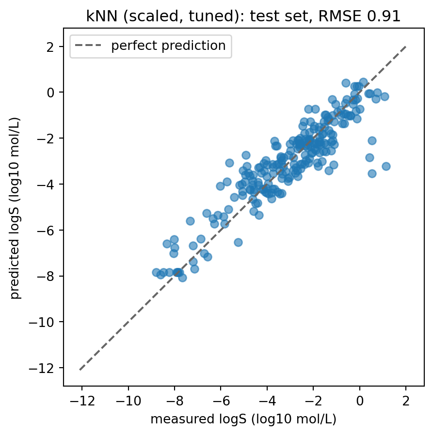
Use best_model, already selected by training CV in Task 7. Store its test predictions in pred_best and draw a parity plot: measured logS on the x axis, predicted on the y axis, with the diagonal y = x. Label the axes with units.
# Task 8: parity plot (measured vs predicted logS) for the model already selected by training CVpred_best = best_model.predict(X_test)fig, ax = plt.subplots(figsize=(5, 5))lims = [y.min() -0.5, y.max() +0.5]ax.scatter(y_test, pred_best, alpha=0.6)ax.plot(lims, lims, linestyle="--", color="0.4", label="perfect prediction")ax.set(xlabel="measured logS (log10 mol/L)", ylabel="predicted logS (log10 mol/L)", title=f"{best_name}: test set, RMSE {results.loc[best_name, 'test RMSE']:.2f}")ax.legend()plt.show()
assertlen(pred_best) ==len(y_test), "pred_best must have one prediction per test molecule"assert root_mean_squared_error(y_test, pred_best) <1.0, "pred_best should come from the best model (test RMSE < 1.0)"print(f"✅ Task 8: best model is '{best_name}'")
✅ Task 8: best model is 'kNN (scaled, tuned)'
Task 9: the ten worst-predicted molecules
Build a DataFrame worst with the columns Compound ID, smiles, measured, predicted and residual (measured − predicted) for the test molecules, sorted by absolute residual, and keep the ten largest. Then look at the SMILES. Do the badly predicted molecules have something in common that the five descriptors cannot see?
# Task 9: the 10 test molecules with the largest absolute residual, with names and SMILESworst = ( esol.loc[X_test.index, ["Compound ID", "smiles"]] .assign(measured=y_test, predicted=pred_best, residual=y_test - pred_best) .sort_values("residual", key=np.abs, ascending=False) .head(10))worst.round(2)
index
Compound ID
smiles
measured
predicted
residual
1064
vamidothion
CNC(=O)C(C)SCCSP(=O)(OC)(OC)
1.14
-3.22
4.37
292
Dimecron
CCN(CC)C(=O)C(=CCOP(=O)(OC)OC)Cl
0.52
-3.53
4.05
796
Triethyl phosphate
CCOP(=O)(OCC)OCC
0.43
-2.83
3.26
758
Acephate
COP(=O)(NC(C)=O)SC
0.54
-2.10
2.64
96
Chlorothalonil
c1(C#N)c(Cl)c(C#N)c(Cl)c(Cl)c(Cl)1
-5.64
-3.06
-2.58
548
Hexachloro-1,3-butadiene
ClC(=C(Cl)C(=C(Cl)Cl)Cl)Cl
-4.92
-2.74
-2.18
436
Diethyl sulfide
CCSCC
-1.34
-3.41
2.07
174
cycloheximide
CC1CC(C)C(=O)C(C1)C(O)CC2CC(=O)NC(=O)C2
-1.13
-3.16
2.03
963
difluron
Fc1cccc(F)c1C(=O)NC(=O)Nc2ccc(Cl)cc2
-6.02
-4.09
-1.93
218
Carbophenthion
CCOP(=S)(OCC)SCSc1ccc(Cl)cc1
-5.74
-3.90
-1.83
assertlen(worst) ==10, "keep exactly the ten worst molecules"assert {"Compound ID", "smiles", "measured", "predicted", "residual"} <=set(worst.columns), "missing columns"assert worst["residual"].abs().is_monotonic_decreasing, "sort by absolute residual, largest first"print("✅ Task 9: worst-ten table built; now read the SMILES")
✅ Task 9: worst-ten table built; now read the SMILES
What the solutions found. Four of the ten worst molecules contain a phosphorus ester group (P(=O) or P(=S)): vamidothion, Dimecron (phosphamidon), triethyl phosphate and acephate are all far more soluble than predicted (residuals of +2.6 to +4.4 log units). The over-predicted group is polyhalogenated: chlorothalonil (four chlorines), hexachloro-1,3-butadiene, difluron and carbophenthion are less soluble than predicted. Neither pattern is visible to the five descriptors, which count rings, rotatable bonds, donors and polar surface area but know nothing about which elements are present or how lipophilic the molecule is. A lipophilicity term (logP) or a fingerprint that sees the phosphate and the halogens would be the next feature to add, which is exactly what Part II does.
Task 10: conclusion
Complete the template below with your own numbers and observations (three to six sentences).
Conclusion. On a held-out test set of ___ molecules, the best model was ___ with a test RMSE of ___ logS (MAE , R² ), compared with ___ for the mean baseline and ___ for linear regression. Cross-validation and test scores agreed to within , so the evaluation looks honest. The largest errors were molecules containing , which suggests the descriptors are missing . A next step would be .
Conclusion (solutions). The model selected by training cross-validation was a scaled k-nearest-neighbours regressor with \(k = 7\), with a test RMSE of 0.91 logS on 226 held-out molecules (MAE 0.68, R² 0.82), compared with an RMSE of 2.17 for the mean baseline and 1.21 for linear regression; ridge regression (best \(\alpha = 10\)) made little difference with these five descriptors. For the three learned models, cross-validation and test RMSE agreed to within about 0.03 logS, a useful consistency check alongside the training-only model selection. The largest errors were organophosphorus esters (under-predicted by 2.6–4.4 log units) and polyhalogenated aromatics and alkenes (over-predicted by about 2), which suggests the five whole-molecule descriptors are missing element-specific and lipophilicity information. A next step would be to add a calculated logP and a structural fingerprint, and to re-evaluate on a scaffold split, since a random split can place close analogues in both training and test sets.
Optional extension (★★★): soluble or not?
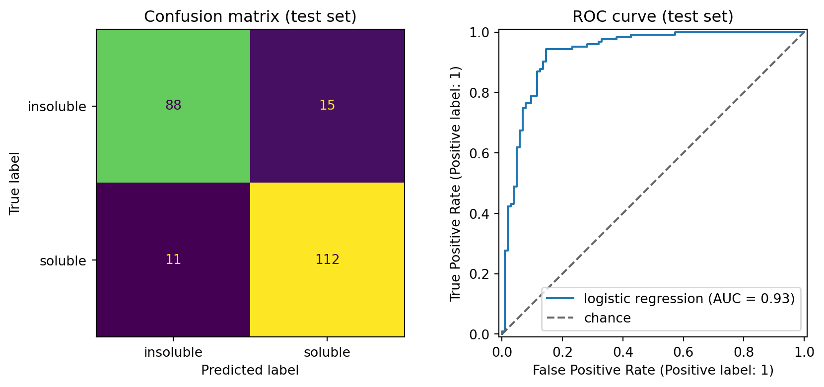
Many projects need a yes/no answer rather than a number. Define “soluble” as logS > −3 (a conventional cut-off used in several solubility papers, not a standard), build a scaled LogisticRegression pipeline on the same train/test split, and evaluate it with a confusion matrix, accuracy, and a ROC curve with its AUC. Compare the accuracy with a DummyClassifier(strategy="most_frequent") baseline.
asserthasattr(clf, "predict_proba"), "clf must be a fitted classifier pipeline"assert clf.score(X_test, y_test_cls) >0.8, "logistic regression should reach well over 80% accuracy"assert auc >0.85, "ROC AUC should be above 0.85"print("✅ Extension: classifier beats the majority-class baseline")
✅ Extension: classifier beats the majority-class baseline
The classes are nearly balanced at this cut-off (about half of the molecules are “soluble”), so the majority baseline is only about 54% and the logistic model’s ~88% accuracy and AUC of about 0.93 are a real gain. Look at the confusion matrix: are the mistakes symmetric, or does the model prefer one kind of error? If this were a screening cascade, which error would be more expensive?
Reflection questions
The CV RMSE and the test RMSE agreed closely for every model. Describe one mistake in the workflow (not in the model) that would have made the test RMSE better than the CV RMSE, and explain why that would be a warning sign rather than good news.
kNN beat the linear models comfortably. Episode 2.6 showed that kNN is also the model most helped by duplicates and near-duplicates across the split. How would you check whether ESOL’s test set contains close analogues of training molecules, and what split would you use to find out how the model does on genuinely new chemistry?
The worst-predicted molecules shared chemical features the descriptors cannot represent. Propose two new features (or one new representation) and say, for each, what kind of error you would expect it to fix and what it might make worse.