2.8 Hyperparameter tuning and honest model selection

45 min of teaching25 min of exercisesbeginner

Questions this episode answers

Which model settings should I search, and how wide should the search be?
When should I use grid search, random search or nested cross-validation?
What should I report after selecting the best model?

What you will be able to do

Distinguish learned parameters from hyperparameters and define a finite search budget.
Search pipeline settings with GridSearchCV and RandomizedSearchCV.
Inspect cv_results_ for sensitivity, timing and boundary winners.
Evaluate a complete model-family search with nested cross-validation.
Refit a selected pipeline and report a final test result without further tuning.

Your solubility model has a regularisation setting called alpha. Your colleague suggests using nearest neighbours instead, which brings a different setting, n_neighbors. Trying both on the test set and keeping the smaller RMSE feels efficient. It also spends the evidence you needed for an honest final report. The solution is to make the search itself a reproducible training procedure, then evaluate that procedure on data it did not use to choose anything.

This lesson builds on the split design in episode 2.7. The example is deliberately small enough to inspect: ridge and kNN on the same ESOL descriptors. In Chapter 3, you will reuse the workflow with trees, ensembles and support vector machines rather than inventing new evaluation rules for each algorithm.

Parameters are learned; hyperparameters configure learning

A parameter is estimated during fitting: the coefficients in ridge regression, for example. A hyperparameter controls the fitting procedure or model structure: ridge’s alpha, a tree’s maximum depth, or a neural network’s learning rate. You choose candidate settings; each candidate then learns its own parameters from a training fold.

Choice	Role	How it is determined
Ridge coefficient for molecular weight	Parameter	Fitted from training features and targets
Ridge `alpha`	Hyperparameter	Compared using development validation scores
Mean used by `StandardScaler`	Fitted preprocessing statistic	Estimated separately in every training fold
Imputation strategy or number of selected features	Preprocessing hyperparameter	Chosen inside model selection
Test split and primary metric	Experimental design	Defined from intended use before the search

Some settings are engineering choices, such as a convergence tolerance or a generous iteration limit. They still need recording, but a solver that has not converged needs diagnosis, not a misleading comparison against converged fits. A random seed records randomness; choosing the seed that produces the best score is another form of selection.

Chemist's corner

Think of a search as comparing experimental protocols. The settings are protocol choices; the fitted coefficients are the result of running a protocol on training measurements. Choosing a protocol and verifying it on the same measurements overstates its reliability. You need separate validation for choosing and evaluation for the final claim.

Write a search plan before running it

For this benchmark, predict measured logS from five available descriptors. Use RMSE as the primary selection metric because large errors deserve extra weight, while also reporting MAE at the end. Retain the existing 80/20 teaching split and use five shuffled folds only within its training portion. This preserves comparison with earlier lessons; as discussed in episode 2.6, a random ESOL split does not establish transfer to novel chemistry.

from pathlib import Path
import numpy as np
import pandas as pd
from sklearn.model_selection import KFold, train_test_split

url = "https://deepchemdata.s3-us-west-1.amazonaws.com/datasets/delaney-processed.csv"
path = Path("data/esol.csv")
esol = pd.read_csv(path if path.exists() else url)
features = ["Molecular Weight", "Number of H-Bond Donors", "Number of Rings",
            "Number of Rotatable Bonds", "Polar Surface Area"]
X, y = esol[features], esol["measured log solubility in mols per litre"]
X_train, X_test, y_train, y_test = train_test_split(
    X, y, test_size=0.2, random_state=42
)
cv = KFold(n_splits=5, shuffle=True, random_state=42)
print(f"Search on {len(X_train)} rows; reserve {len(X_test)} rows")

Search on 902 rows; reserve 226 rows

Choose ranges from how a setting works. Positive scale parameters often need multiplicative steps: alpha values 0.001, 0.01, 0.1, 1, 10, 100 and 1,000 explore different orders of magnitude. A uniform sequence from 0 to 1,000 barely examines small penalties. Counts such as neighbours need sensible integer values; k must not exceed the size of the smallest training fold.

Keep an explicit compute budget. Seven alpha values with five folds require 35 fits, plus one refit of the selected configuration on all development rows. A grid with 7 × 8 × 6 combinations would require 1,680 fold fits. Search size grows multiplicatively, even when most combinations are uninteresting.

A small grid you can inspect

from sklearn.linear_model import Ridge
from sklearn.pipeline import Pipeline
from sklearn.preprocessing import StandardScaler
from sklearn.model_selection import GridSearchCV

pipeline = Pipeline([("scale", StandardScaler()), ("model", Ridge())])
ridge_grid = {"model__alpha": np.logspace(-3, 3, 7)}
ridge_search = GridSearchCV(
    pipeline, ridge_grid, cv=cv, scoring="neg_root_mean_squared_error",
    return_train_score=True, error_score="raise", n_jobs=1,
)
ridge_search.fit(X_train, y_train)
print(ridge_search.best_params_)
print(f"Selection CV RMSE: {-ridge_search.best_score_:.3f} log10 mol/L")

{'model__alpha': np.float64(10.0)}
Selection CV RMSE: 1.188 log10 mol/L

The two underscores in model__alpha mean “the alpha setting of the step named model”. GridSearchCV clones the whole pipeline for each candidate and fold. That is why the scaler cannot see the validation rows during fitting. The default refit=True then fits the winning pipeline on all X_train, which makes ridge_search.predict(...) available.

Predict before you run

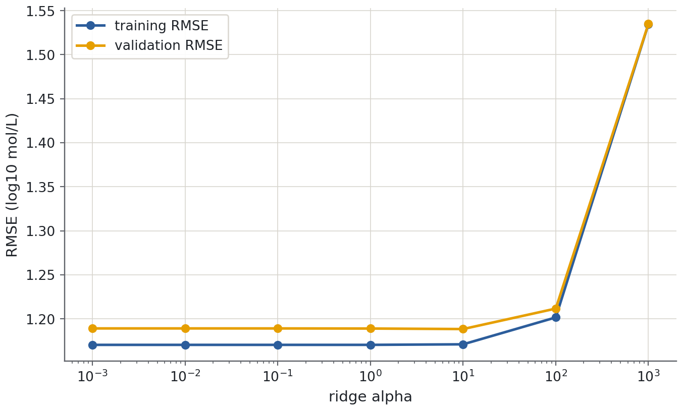
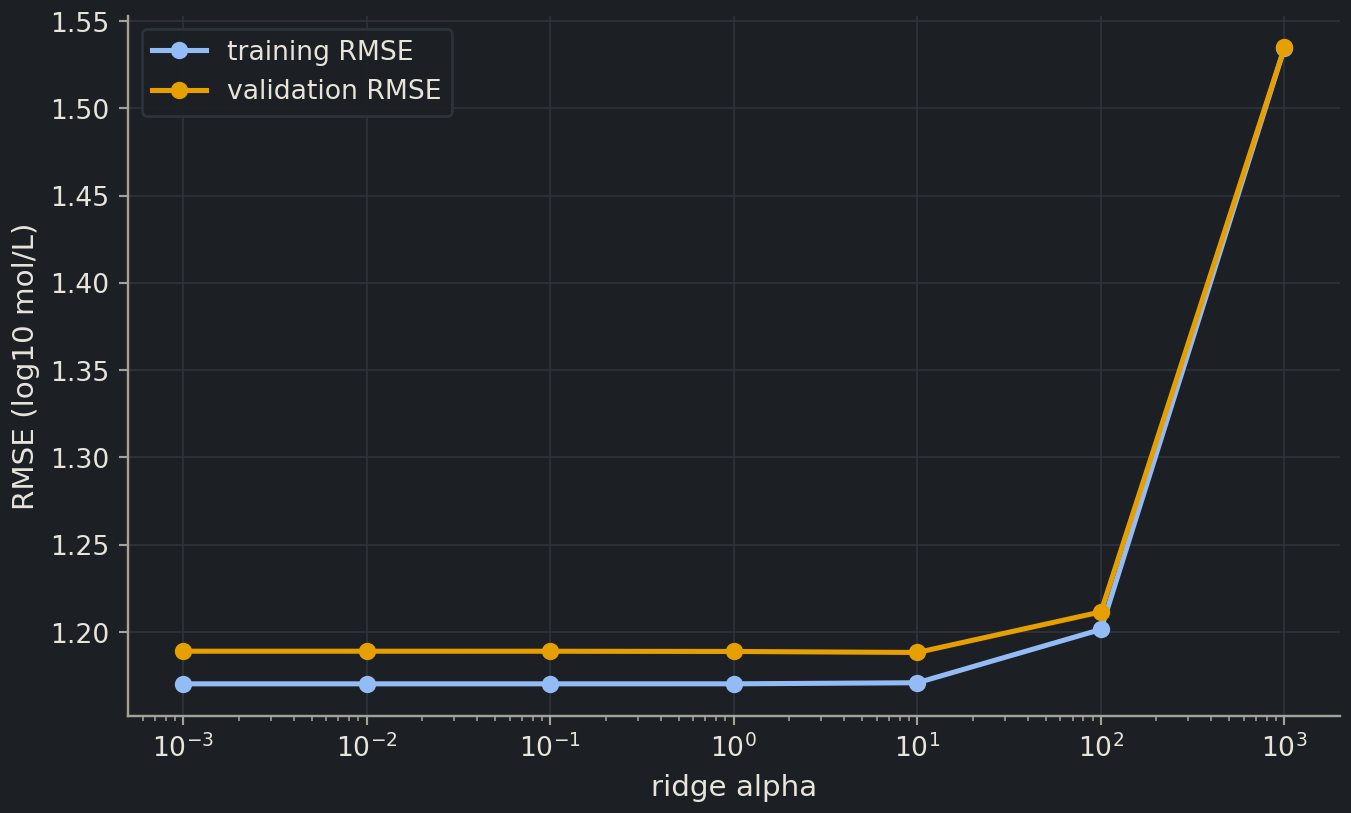
If several alphas produce almost identical validation errors, will best_params_ tell you that the evidence is weak? Predict what the full table will show that the single winning parameter cannot.

results = pd.DataFrame(ridge_search.cv_results_)
results["validation RMSE"] = -results["mean_test_score"]
results["training RMSE"] = -results["mean_train_score"]
results[["param_model__alpha", "training RMSE", "validation RMSE",
         "std_test_score", "mean_fit_time"]].round(4)

index	param_model__alpha	training RMSE	validation RMSE	std_test_score	mean_fit_time
0	0.001	1.1703	1.1890	0.0978	0.0064
1	0.010	1.1703	1.1890	0.0978	0.0029
2	0.100	1.1703	1.1890	0.0978	0.0027
3	1.000	1.1704	1.1889	0.0979	0.0028
4	10.000	1.1710	1.1883	0.0985	0.0028
5	100.000	1.2015	1.2116	0.1047	0.0027
6	1000.000	1.5347	1.5349	0.1219	0.0028

best_params_ must name a winner even when the numerical differences are tiny. Read the neighbouring scores, the training–validation gap and fitting time. A broad flat region suggests the exact setting is not crucial on this benchmark. Large penalties eventually underfit. Do not promote a thousandth-of-a-unit advantage into a claim that one alpha is scientifically optimal.

import matplotlib.pyplot as plt

fig, ax = plt.subplots()
for label in ["training RMSE", "validation RMSE"]:
    ax.plot(results["param_model__alpha"].astype(float), results[label], marker="o", label=label)
ax.set(xscale="log", xlabel="ridge alpha", ylabel="RMSE (log10 mol/L)")
ax.legend()
plt.show()

Training and validation RMSE across ridge alpha on a logarithmic axis, showing whether the minimum is broad or sensitive to regularisation.

If the best setting lies at a boundary and the validation trend is still improving, consider extending the range using development data only. Log the extension: adapting the search is still model selection. More attempts increase the opportunity to exploit noise in the validation scores; an untouched final evaluation becomes more valuable, not less.

Random search gives a direct budget

random search samples candidate configurations instead of evaluating every grid combination. It is useful when several settings span wide ranges and you can afford only a fixed number of trials. A logarithmic sampling distribution gives comparable attention to each order of magnitude of a positive scale parameter.

from scipy.stats import loguniform
from sklearn.model_selection import RandomizedSearchCV

random_search = RandomizedSearchCV(
    pipeline, {"model__alpha": loguniform(1e-3, 1e3)},
    n_iter=8, cv=cv, scoring="neg_root_mean_squared_error",
    random_state=42, error_score="raise", n_jobs=1,
)
random_search.fit(X_train, y_train)
print(random_search.best_params_)
print(f"Selection CV RMSE: {-random_search.best_score_:.3f}")

{'model__alpha': np.float64(3.907967156822881)}
Selection CV RMSE: 1.189

Here n_iter=8 means 40 fold fits plus a refit. With one parameter and a small grid, random search has little practical advantage; this cell shows the interface you will use for larger spaces. Sampling cannot guarantee a global optimum. A reproducible seed makes the sampled candidates repeatable, while a recorded distribution explains what was explored.

Other methods include successive halving, which allocates more resources to promising configurations, and Bayesian optimisation, which uses previous trials to propose new ones. They are useful extensions when fits are expensive. They do not remove the need for appropriate splits, a fixed objective or independent evaluation. For a small first project, an understandable modest search is enough.

Compare model families inside the search

Selecting ridge versus kNN is a hyperparameter decision at a higher level. Use a list of dictionaries so each family receives only relevant settings. Ridge has alpha; kNN has n_neighbors and weights. The same scale step is appropriate for both.

from sklearn.neighbors import KNeighborsRegressor

family_grid = [
    {"model": [Ridge()], "model__alpha": [0.01, 1.0, 100.0]},
    {"model": [KNeighborsRegressor()], "model__n_neighbors": [3, 9, 21],
     "model__weights": ["uniform", "distance"]},
]
search = GridSearchCV(
    pipeline, family_grid, cv=cv, scoring="neg_root_mean_squared_error",
    error_score="raise", n_jobs=1,
)
search.fit(X_train, y_train)
print(search.best_params_)
print(f"Selected family CV RMSE: {-search.best_score_:.3f}")

{'model': KNeighborsRegressor(), 'model__n_neighbors': 9, 'model__weights': 'distance'}
Selected family CV RMSE: 0.889

The grid has nine configurations, not every possible cross-product across both dictionaries. Its winning CV score answered which of these candidates should I select? It is optimistic if reused as the independent answer to how good is the selection procedure? The same principle applies when choices were made by hand across many notebooks rather than by one search object.

Common mistake

The best model is conditional on the search

“Best” means best mean validation score among these candidates, on these features, folds and metric. A different representation or an unseen scaffold may change the ranking. Report the search space so the claim is interpretable, and compare to a simple baseline before treating a sophisticated winner as useful.

Nested CV evaluates the complete procedure

nested cross-validation adds an outer loop. For each outer split, it gives the inner search only the outer training rows. The search chooses its settings using inner validation folds, refits on those outer training rows, and predicts the outer held-out rows. Neither the scaler nor the family choice sees the outer validation labels.

from sklearn.model_selection import cross_validate

outer = KFold(n_splits=3, shuffle=True, random_state=42)
nested = cross_validate(
    search, X_train, y_train, cv=outer,
    scoring="neg_root_mean_squared_error", return_estimator=True,
    error_score="raise", n_jobs=1,
)
outer_rmse = -nested["test_score"]
print("Outer-fold RMSE:", outer_rmse.round(3))
print(f"Mean {outer_rmse.mean():.3f}; fold SD {outer_rmse.std(ddof=1):.3f}")

Outer-fold RMSE: [0.947 0.92  0.886]
Mean 0.918; fold SD 0.030

We use three outer folds to keep the example quick. There are 3 × (9 × 5 + 1) fits: inner searches plus refits. Only the outer-fold scores evaluate the search. They estimate the procedure trained on the smaller outer training sets; they are not a guarantee for the particular final refit. As in episode 2.7, the fold SD is descriptive variability, not a confidence interval.

for fold, fitted_search in enumerate(nested["estimator"], start=1):
    print(f"Outer fold {fold}: {fitted_search.best_params_}")

Outer fold 1: {'model': KNeighborsRegressor(), 'model__n_neighbors': 9, 'model__weights': 'distance'}
Outer fold 2: {'model': KNeighborsRegressor(), 'model__n_neighbors': 9, 'model__weights': 'distance'}
Outer fold 3: {'model': KNeighborsRegressor(), 'model__n_neighbors': 9, 'model__weights': 'distance'}

Different outer folds can choose different settings or even families. That reflects selection instability; it is not a reason to take the settings from whichever outer fold scored best. To build the final model, run the declared search on all development rows, as search.fit(X_train, y_train) already did above.

If you have no separate test set, nested CV can be the final evaluation of a predefined selection procedure. If you repeatedly revise the procedure after viewing outer results, the outer loop also becomes development. Likewise, if you compare many independently nested searches and only report the best outer score, the family-selection optimism has moved outward. Here the family choice is inside each inner search, and a reserved test set remains available.

For grouped or temporal data, both loops must respect the scientific split constraint. Do not silently use random inner folds for a grouped scientific question; group identifiers must reach the inner splitter too. A small explicit loop is often clearer than complicated metadata routing. Lab 3 practises a complete nested comparison.

Refit, evaluate and stop choosing

All choices are now fixed. Fit a mean baseline on development data and evaluate it alongside the selected pipeline. The grid and random-search demonstrations above do not compete for this final report: the declared family grid is the procedure being assessed.

from sklearn.dummy import DummyRegressor
from sklearn.metrics import mean_absolute_error, root_mean_squared_error, r2_score

baseline = DummyRegressor().fit(X_train, y_train)
report = []
for name, model in [("mean baseline", baseline), ("selected pipeline", search)]:
    prediction = model.predict(X_test)
    report.append({"model": name, "MAE": mean_absolute_error(y_test, prediction),
                   "RMSE": root_mean_squared_error(y_test, prediction),
                   "R2": r2_score(y_test, prediction)})
pd.DataFrame(report).set_index("model").round(3)

index	MAE	RMSE	R2
model	index	index	index
mean baseline	1.732	2.174	-0.000
selected pipeline	0.622	0.895	0.831

State the test metrics with their units, the baseline, sample counts, feature definitions, split design, search space, selected settings and software versions. Save the whole fitted pipeline, not just the final estimator; preprocessing is part of the model. The reproducibility toolkit gives a short report template.

A disappointing result is still a result. Investigate it honestly, but label the investigation as new development and obtain fresh evaluation before claiming improvement. After the evaluation, you may train a deployment model on all available data if that is the intended use; the old test score then describes the earlier evaluated procedure, not a fresh independent test of the all-data fit.

Exercises

Exercise★☆☆

Count the fits

A grid has four depths and three leaf sizes, with five inner folds and four outer folds. Each search refits its winner. How many fits does nested CV require, before a final all-development search?

SolutionShow solution

There are 4 × 3 = 12 candidates, 12 × 5 = 60 inner fold fits, and one refit per outer fold. Four outer folds therefore require 4 × 61 = 244 fits. A final search adds another 61. Preprocessing is refitted as part of each pipeline fit.

Exercise★★☆

Debug this search

Someone runs GridSearchCV(Ridge(), {"alpha": [0.1, 1, 10]}) on a table scaled before splitting, then reports best_score_ as “test RMSE”. Identify three errors.

SolutionShow solution

The scaler leaked held-out information: put it inside a pipeline. The default regressor score is R², not RMSE: request scoring="neg_root_mean_squared_error" and negate once. The winning CV score selected the configuration: evaluate the fixed winner on untouched data or evaluate the complete search with outer CV. Pipeline parameters must then be addressed by their step names.

Exercise★★★

A constrained search decision

The best RMSE is 0.94 for a slow candidate and 0.95 for a much faster one. Fold results vary substantially and the application needs interactive predictions. What should you do before opening the test set?

SolutionShow solution

Inspect paired fold results and measure prediction latency under realistic conditions; fitting time is not prediction time. Apply a declared trade-off, such as choosing the faster model among candidates within a scientifically acceptable error tolerance. Record that rule and the selected configuration before final testing. A 0.01 mean difference alone neither proves superiority nor establishes equivalence.

Where this is going

Lab 2 assembles a complete first project, while Chapter 3 expands the candidate families. Chapter 4 adds learning rates, batch sizes and stopping epochs to the choices; they belong inside the same separation between development and final evaluation.

See the scikit-learn search guide for search APIs and the nested-CV example for the distinction between selecting and assessing a procedure.

Key points

A search is an experiment: specify the metric, split design, candidates and compute budget before running it.
Use logarithmic ranges for positive scale parameters such as regularisation strength.
Grid search covers a small explicit set; random search samples a fixed number of configurations.
best_score_ is a selection score, not an independent estimate of final performance.
Nested CV places the entire selection procedure inside each outer training fold.
Model family, preprocessing, feature selection, thresholds and stopping decisions all belong inside development.