How can I view thirty measurements on a two-dimensional plot?
Does retaining most of the variance retain the information needed to predict?
What you will be able to do
Fit a scaled PCA and interpret scores, component weights and explained variance.
Distinguish exploratory visualisation from validated predictive preprocessing.
Place PCA inside a cross-validated classification pipeline.
The breast-cancer teaching dataset has thirty measurements per sample. A scatter plot can show two at a time, but hundreds of possible pairs make it hard to see the overall arrangement. Principal component analysis (PCA)principal component analysisAn unsupervised projection onto orthogonal directions of greatest input variance. constructs new coordinates that summarise variation across the original measurements. It lets us ask whether samples lie along a few dominant directions without using the diagnosis to construct those directions.
PCA is unsupervised learningunsupervised learningFinding structure in data that has no labels, such as clusters or low-dimensional summaries.. It answers a question about the feature table, not “which measurements best predict the label?” A prominent direction might represent size, biological heterogeneity, an instrument effect or a batch difference. The algorithm alone cannot tell us which interpretation is correct.
Rotate the coordinate system, then discard directions
Imagine a cloud of points shaped like a long, narrow ellipse. The horizontal and vertical axes may describe the same movement redundantly. Rotate the axes so that one points along the long direction, and most variation can be expressed by a single coordinate. PCA generalises this construction to many features.
The first principal componentprincipal componentA direction, and its corresponding scores, in the coordinate system learned by PCA. is the direction with greatest variance. The next captures the greatest remaining variance while being perpendicular to the first, and so on. Each new coordinate, or score, is a weighted sum of centred features. Those weights describe a direction; they are not coefficients fitted to predict the target.
For centred and standardised row \(z_i\), the first score is
\[t_{i1} = z_i^\mathsf{T} v_1.\]
Here \(v_1\) is a unit-length vector of component weights. Retaining two components gives every observation two scores for plotting. Discarding the other components loses variation; no two-dimensional picture can promise to preserve every important relationship among thirty-dimensional observations.
Maths corner
PCA’s directions are eigenvectors of the sample covariance matrix; their eigenvalues are the variances along those directions. A singular value decomposition obtains the same directions without explicitly constructing the covariance matrix. The implementation handles this algebra. What you must choose is the representation, scaling and number of retained dimensions.
Start with development data
We reserve a stratified test set before looking for patterns. Stratification preserves approximate class proportions; it does not address repeated patients or batch relationships. This dataset is used as an educational example, not as a validated clinical tool.
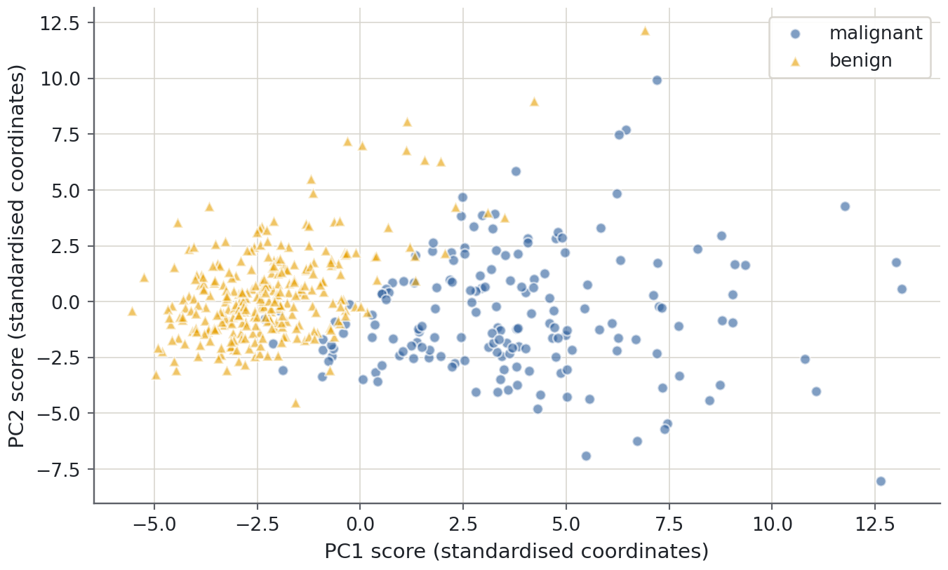
Read the mapping rather than guessing: class 0 is malignant and class 1 is benign in this dataset. The plot labels will use those names. Neither class is supplied to the PCA fit; we may later colour the plot by diagnosis to describe an association.
Measurements have different scales: area and smoothness are not directly comparable numeric quantities. Standardisation gives each feature unit variance on the development data before PCA. That is appropriate for this introductory comparison, but not mandatory for every scientific use of PCA. If absolute measurement variation is meaningful, preserving original units may be deliberate.
from sklearn.decomposition import PCAfrom sklearn.pipeline import make_pipelinefrom sklearn.preprocessing import StandardScalerprojection = make_pipeline(StandardScaler(), PCA(svd_solver="full"))scores = projection.fit_transform(X_train)pca = projection.named_steps["pca"]print(f"First two components retain {pca.explained_variance_ratio_[:2].sum():.1%} of variance")
First two components retain 63.4% of variance
PCA itself centres but does not standardise its inputs, so the explicit scaler is necessary for this chosen geometry. components_ stores unit component directions, and explained_variance_ratio_ reports each direction’s share of the fitted input variance. These attribute definitions are documented in the PCA API.
Read the map without overclaiming
Predict before you run
If the first two components retain a large fraction of variance, must the diagnosis classes separate on the plot? Give a counterexample before looking.
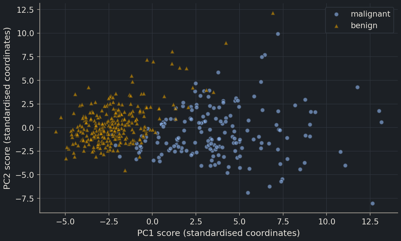
A visible association with diagnosis can be useful, but this is a development-data description. It does not estimate classification accuracy on new patients. Conversely, overlap in two components does not prove prediction is impossible: discarded directions or nonlinear relationships may contain useful information.
Outliers deserve investigation. A distant point can reflect an unusual sample, a measurement error or a meaningful subgroup. Automatically deleting it because it spoils the plot risks removing precisely the cases the model must handle. Check the original measurements and their provenance before deciding what to do.
How much variation remains?
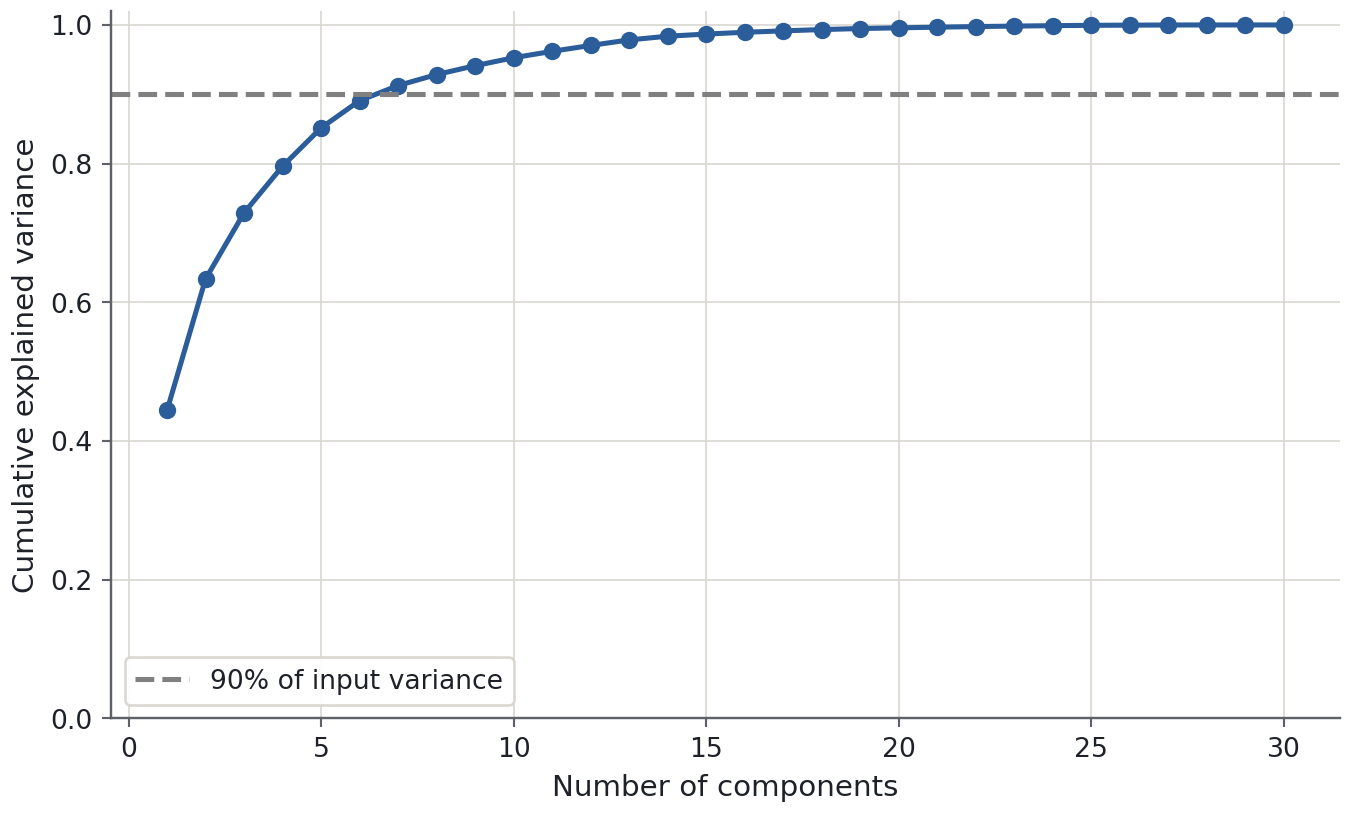
A scree plot shows variance contributed by each component; a cumulative plot shows the total retained as components are added. A sharp bend can suggest a compact representation, but it is a heuristic. There need not be a unique correct number of components.
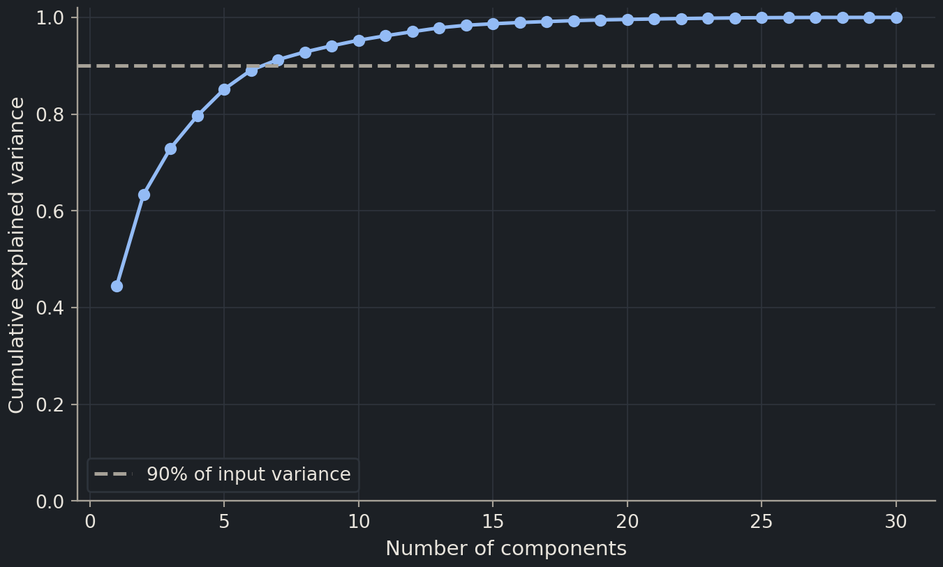
Variance is not signal by definition. A high-variance direction could track instrument brightness while a low-variance direction distinguishes a disease subtype. Retaining 90% of variance can be sensible for compression, but does not guarantee retaining 90% of the useful predictive information. To use PCA for prediction, choose the dimension count by an appropriate development metric inside the pipeline.
mean concave points     0.261
mean concavity          0.258
worst concave points    0.250
mean compactness        0.242
worst perimeter         0.235
worst concavity         0.230
mean perimeter          0.226
worst radius            0.226
Name: PC1 weight, dtype: float64
Large absolute weights identify measurements contributing strongly to this direction in standardised units. The signs show which measurements move together or oppositely along that axis. Correlated radius, perimeter and area features can jointly describe size, but that interpretation should come from the listed measurements, not from naming every first component “size”.
The sign of a whole component is arbitrary: multiplying all weights and all scores by −1 describes the same geometry. A left-to-right reversal in another implementation is not a biological disagreement. Terminology also varies: some sources call these unit direction weights “loadings”, while others reserve that word for weights multiplied by the square root of the eigenvalue. State what numbers you are reporting.
Common mistake
Unsupervised preprocessing can still leak
Fitting PCA on every sample uses the validation and test feature distributions, even without their labels. If the components then feed a predictive model, the evaluation no longer represents learning the entire procedure from training data alone. Put PCA inside the cross-validation pipeline, just like the scaler.
Reconstruction clarifies what compression preserves
Projecting a standardised observation onto the first \(k\) directions and mapping it back gives an approximation of the original feature vector. With directions stored in columns of \(V_k\), the reconstruction is \(\hat z_i = V_k V_k^\mathsf{T} z_i\). Add the fitted means and undo standardisation to express that approximation in the original measurement units. Discarded directions explain the difference between the measured row and its reconstruction.
PCA chooses its retained linear subspace to minimise squared reconstruction error for the fitted, centred table. This gives a precise meaning to “preserving information”: it preserves variation measured by that particular squared-distance objective. It does not know which reconstruction errors matter for diagnosis. A small change in one low-variance feature may be decisive for a downstream label even when its contribution to total reconstruction error is tiny.
Think of two tasks with the same measurements. For a compact visual summary, two components may be a reasonable compromise that makes the main cloud visible. For archiving measurements, a higher variance-retention threshold may be needed. For predicting a target, the dimension count is a model hyperparameter chosen by predictive validation, with a no-PCA option kept as a baseline. The correct compression level depends on the intended use.
A large reconstruction error can also flag an unusual observation relative to the fitted subspace, but it is not a universal anomaly detector. A sample can lie far along a retained component and still reconstruct well, while a legitimate rare sample can reconstruct poorly. Any rule that flags samples from reconstruction error needs its own development threshold and independent evaluation against the intended scientific definition of an anomaly.
Evaluate PCA as part of a classifier
Compare a few dimension counts and an option to skip PCA. The identical pipeline structure ensures both standardisation and the component fit happen within each fold. Balanced accuracy averages sensitivity across the two classes; it is used here as a simple development metric, not a complete assessment of clinical usefulness.
{'pca__n_components': 10}
Selected development balanced accuracy: 0.979
Keeping all original features is a legitimate result. PCA may help with redundancy, noise, storage or visualisation, but reducing dimensions is not automatically an improvement. The selected CV score has participated in a decision, so it must not be presented as the final independent evaluation. Keep the reserved test closed until the full classification procedure is fixed.
Exercises
Exercise★☆☆
What did 90% mean?
A colleague says “our first five components explain 90% of the variance, so the classifier will be 90% accurate.” What is wrong?
SolutionShow solutionHide solution
Explained variance concerns how much variation in the input coordinates is retained. Classification accuracy concerns agreement with labels on unseen observations. PCA did not optimise label prediction, and there is no conversion from one percentage to the other.
Exercise★★☆
Project genuinely new rows
Without refitting, project the first three reserved feature rows with the exploratory projection object. Why must you use transform rather than fit_transform?
transform uses the development means, scales and axes. Refitting would create a different coordinate system. This demonstrates applying a fixed transformation; it does not use the reserved labels or compare candidate models. In a final modelling workflow, apply the complete chosen prediction pipeline directly.
Exercise★★★
A batch-shaped map
PC1 separates samples almost perfectly by laboratory, and most cases were measured in one laboratory while most controls were measured in the other. Would the class-coloured map demonstrate a disease signature?
SolutionShow solutionHide solution
No. Laboratory and diagnosis are confounded, so the map cannot separate their contributions. Inspect metadata, improve the study design and evaluate across laboratories or batches. Simply removing PC1 may also remove biological signal and is not a substitute for resolving the confounding.
Where this is going
Clustering assigns groups in a chosen feature geometry, while PCA provides a lower-dimensional view of that geometry. Both become common tools for gene-expression and sequence-derived features in Part III. Their plots are starting points for hypotheses; evidence about predictive performance or biological mechanisms requires additional evaluation.
Key points
PCA finds orthogonal directions of high input variance without using the target.
Scale deliberately: PCA centres features but does not automatically standardise their units.
Explained variance measures retained input variation, not predictive accuracy.
When PCA is part of prediction, fit both scaling and PCA inside each training fold.