import torch

w = torch.tensor(1.0, requires_grad=True)
loss = (2 * w - 6) ** 2
loss.backward()
print("loss:", loss.item(), "gradient:", w.grad.item())
loss: 16.0 gradient: -16.0A calibration line relates an instrument signal to a known concentration. In Chapter 2 you fitted a line by writing its gradient explicitly. A neural network replaces that line with a composition of many operations, but the fitting principle is unchanged: calculate how changing each parameter affects the loss, then take a small step that reduces it.
autogradautogradAutomatic differentiation through the tensor operations that produced a result. is automatic differentiation. It tracks the operations used to produce a result and applies the chain rule to obtain derivatives. It does not search for an algebraic expression in a textbook, estimate every derivative by numerical perturbation, or decide whether your scientific question is sensible. It differentiates the calculation you actually wrote, including mistakes.
Suppose a one-parameter model predicts twice its weight, and the measured value is six. Its squared-error loss is \(L(w)=(2w-6)^2\). At \(w=1\), the prediction is two, the loss is 16, and the derivative is \(4(2w-6)=-16\). A negative derivative means increasing the weight slightly will decrease the loss nearby.
If gradient descent subtracts the gradient multiplied by a positive learning rate, will the first update increase or decrease this weight? What would happen if you added the gradient instead?
import torch
w = torch.tensor(1.0, requires_grad=True)
loss = (2 * w - 6) ** 2
loss.backward()
print("loss:", loss.item(), "gradient:", w.grad.item())loss: 16.0 gradient: -16.0requires_grad=True marks a tensor whose role in the calculation should be tracked. loss.backward() computes derivatives and places the derivative with respect to w in w.grad. The weight is still 1.0: obtaining a gradient and changing a parameter are separate operations. The PyTorch autograd tutorial explains this graph-based calculation.
The loss here is a scalar. Real training losses usually average per-sample losses into one scalar too. Autograd can handle vector outputs, but they require specifying what combination of output derivatives is wanted. Starting with a scalar mean loss keeps the training objective explicit.
Usually the measurements in X and y do not need gradients: you are adjusting the model, not changing the observed experiment. Model parameters do need gradients. There are later applications that differentiate a prediction with respect to an input, such as sensitivity analysis, but that is a separate calculation with a different interpretation. A large input derivative describes local model sensitivity, not the causal effect of changing a molecule or an assay condition. Decide which quantity is allowed to change before marking it for differentiation.
For parameters collected in a vector \(\theta\), backward() computes the components of \(\nabla_\theta L\). Reverse-mode differentiation is efficient when there are many parameters and one scalar loss: it reuses intermediate derivatives while moving backwards through the calculation. You still choose the function \(L\) and the optimiser; differentiation alone solves neither model selection nor optimisation.
The gradient-descent rule is \(w \leftarrow w-\eta\,\partial L/\partial w\), where \(\eta\) is the learning ratelearning rateThe step size of gradient descent; too large diverges, too small crawls.. With a learning rate of 0.1, the first step changes the weight from 1.0 to 2.6. The optimum for this artificial example is 3.0, so the step moves towards it without reaching it.
with torch.no_grad():
    w -= 0.1 * w.grad
print("updated weight:", w.item())
print("new loss:", ((2 * w - 6) ** 2).item())
updated weight: 2.5999999046325684
new loss: 0.6400002837181091The update is inside torch.no_grad() because it is bookkeeping for the learning algorithm, not part of the prediction whose derivative we need next. A new forward calculation will build a new computation graph using the new parameter values. Later, an optimiser will perform this update for us.
The learning rate is a hyperparameter, so choose it using training and validation evidence. A tiny rate may make progress too slow to notice. A large rate can overshoot and increase the loss or make it non-finite. A successful first step does not prove that the same rate will behave well in every part of a larger network’s loss surface.
Autograd adds new derivatives to existing .grad values. This supports deliberate accumulation over several batches, but ordinary training normally wants a fresh gradient for each update. Clearing gradients is therefore part of the loop, not an optional optimisation.
w.grad = None
new_loss = (2 * w - 6) ** 2
new_loss.backward()
print("fresh gradient:", w.grad.item())
fresh gradient: -3.200000762939453The derivative now describes the loss at the updated weight. Without clearing it, the old value of −16 would remain and the new derivative would be added to it. You would no longer be taking the gradient-descent step you intended.
Do not call backward() twice on the same freed graph to fix this. Recompute the forward pass and loss each step. Autograd generally frees intermediates after backward to save memory; retaining graphs is a specialised tool, not a normal requirement for these training loops. Also avoid storing whole loss tensors in a history list: store loss.item() so the history contains ordinary numbers rather than references to training calculations.
Now use a small synthetic calibration experiment. We know the generating relation, so this is a test of the training machinery. It is not a benchmark and its training error must not be presented as evidence of performance on a future assay.
import numpy as np

rng = np.random.default_rng(42)
x_array = np.linspace(-1, 1, 40).reshape(-1, 1)
y_array = 1.5 * x_array[:, 0] - 0.4 + rng.normal(0, 0.08, 40)
X = torch.tensor(x_array, dtype=torch.float32)
y = torch.tensor(y_array, dtype=torch.float32)
torch.manual_seed(42)
model = torch.nn.Linear(1, 1)
print(model)
Linear(in_features=1, out_features=1, bias=True)Linear(1, 1) stores one coefficient and one bias as trainable parameters. Calling model(X) performs the batched linear prediction from the previous episode. The layer starts with initial values; the seed makes that starting point reproducible in the same environment.
loss_fn = torch.nn.MSELoss()
optimiser = torch.optim.SGD(model.parameters(), lr=0.1)
history = []
for step in range(100):
    optimiser.zero_grad(set_to_none=True)
    pred = model(X).squeeze(1)
    loss = loss_fn(pred, y)
    loss.backward()
    optimiser.step()
    history.append(loss.item())
print("weight:", model.weight.item(), "bias:", model.bias.item())
print("first and last training loss:", history[0], history[-1])
weight: 1.5119200944900513 bias: -0.3969387412071228
first and last training loss: 1.7056150436401367 0.004201712552458048Read the loop in order. Clear old gradients, produce predictions, calculate a scalar loss, differentiate it, then update the parameters. model.parameters() tells the optimiser which tensors it owns; it does not supply the data. set_to_none=True clears gradient storage so the next backward pass creates the current gradients.
The learned coefficient should be close to 1.5 and the bias close to −0.4, with some difference caused by the noise and finite training time. The reported final history value is the loss just before the final update. If you need a metric for the final fitted model, compute it afterwards using a fresh forward pass.
import matplotlib.pyplot as plt

fig, ax = plt.subplots()
ax.plot(np.arange(1, len(history) + 1), history)
ax.set(xlabel="gradient updates", ylabel="training MSE (signal units squared)")
plt.show()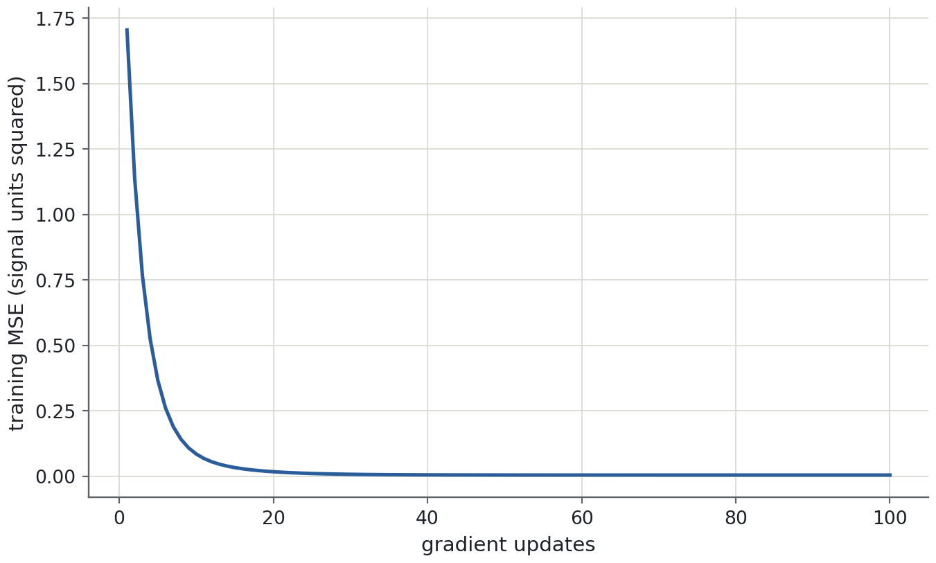
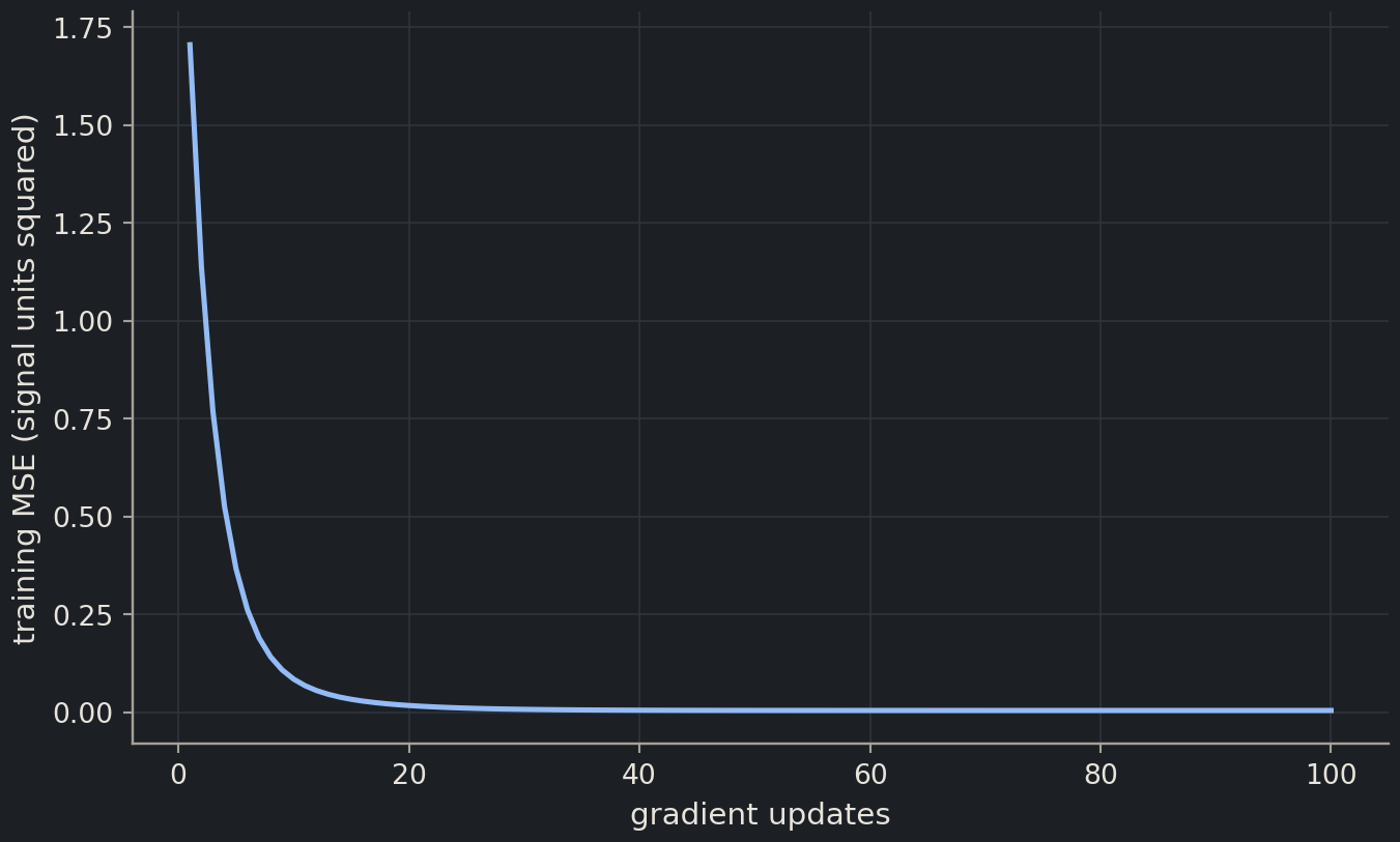
A falling curve means this optimiser is reducing this training objective. It says nothing yet about an unseen sample, whether the labels are correct or whether a linear relation is appropriate outside the observed range. Separate validation will reappear as soon as the models are flexible enough to make those issues easy to miss.
A finite difference estimates a derivative by evaluating the loss a little above and below the parameter. It is useful as a sanity check for a tiny example. It is too expensive to replace autograd for a model with many parameters, and the step size introduces numerical approximation error.
def scalar_loss(value):
    return (2 * value - 6) ** 2

epsilon = 1e-4
finite_difference = (scalar_loss(1 + epsilon) - scalar_loss(1 - epsilon)) / (2 * epsilon)
print("finite-difference derivative:", finite_difference)
finite-difference derivative: -15.999999999980474This agrees with the derivative of −16 above. If a custom scientific loss disagrees with its expected derivative, simplify it before training a large model. Check one scalar, then one sample, then a batch. Shape mistakes, detached tensors and the wrong reduction are easier to diagnose in that order.
Breaking the path from loss to parameters
Converting predictions to NumPy and constructing a fresh tensor for the loss disconnects the calculation. Calling .item() on a training quantity also turns it into an ordinary number. Use these conversions for logging and evaluation; keep the training loss connected to the original model outputs. Do not set requires_grad=True on a detached replacement and expect it to reconnect earlier operations.
Derivative versus update
For \(L(w)=(w-4)^2\) at \(w=1\), calculate the gradient and the next weight for a learning rate of 0.25. Which operation corresponds to backward, and which to step?
The derivative is \(2(w-4)=-6\). The next weight is \(1-0.25(-6)=2.5\). backward calculates −6; step uses that derivative and the learning rate to change the parameter to 2.5. Neither operation examines a validation set or chooses a model architecture.
Debug this: a frozen model
A colleague writes the following loop. Their reported loss never improves. Find the missing operation and explain why gradients alone are insufficient.
for step in range(100):
    optimiser.zero_grad(set_to_none=True)
    loss = loss_fn(model(X).squeeze(1), y)
loss.backward()Add optimiser.step() after loss.backward(). The loop calculates derivatives at the same parameter values every time because it never applies an update. Conversely, calling step() without calculating fresh gradients uses no useful current direction. The optimiser must also own this model’s parameters; creating a new model after creating the optimiser is another way to update the wrong tensors.
Distinguish optimisation from evaluation
The calibration training loss has fallen by a factor of 100. Write two claims this supports and two claims it does not support. Propose one next experiment.
It supports that the parameters changed in a direction that reduced the chosen loss, and that the fitted model describes these training observations better under that metric. It does not establish accuracy on a new instrument or justify extrapolation beyond the measured concentration range. Hold back an independent calibration series, preserve the units and preprocessing, and assess predictions there; use validation, rather than that final series, to adjust learning rate or model complexity.
Episode 4.3 replaces the single line with a small nonlinear network. The same chain rule will train atom-level representations in Chapter 7 and sequence models in Chapter 10. You do not need a new learning principle for each architecture; you need the right input, loss and evaluation experiment.