3.6 Interpreting models without inventing mechanisms

40 min of teaching25 min of exercisesintermediate

Questions this episode answers

Which descriptors does a model rely on for useful predictions?
How does a prediction change when one input changes?
What can a model explanation tell me about causation?

What you will be able to do

Compute and interpret permutation importance on held-out development data.
Read partial dependence and individual conditional expectation plots.
Distinguish global importance, local attribution and causal evidence.

A solubility model performs better than the mean baseline. A chemist now asks, “What has it learned, and what should I change in this molecule?” Those are two different questions. We can inspect the model’s dependence on descriptors; predicting the consequence of a chemical intervention requires additional scientific evidence and assumptions.

An explanation is also conditional on model quality. A poor model can have a beautifully organised importance plot. First establish that predictions are useful under a relevant split, then ask what information supports them. We will interpret one declared forest on a held-out development validation partition and keep the final test set closed.

Keep an interpretation partition inside development

The validation partition may influence hypotheses or feature choices, so it belongs inside the development process. If you subsequently revise the model, evaluate the revised procedure on fresh evidence. Calling a set “test” does not preserve its independence once its outcomes guide decisions.

from pathlib import Path
import numpy as np
import pandas as pd
from sklearn.model_selection import train_test_split

url = "https://deepchemdata.s3-us-west-1.amazonaws.com/datasets/delaney-processed.csv"
path = Path("data/esol.csv")
esol = pd.read_csv(path if path.exists() else url)
features = ["Molecular Weight", "Number of H-Bond Donors", "Number of Rings",
            "Number of Rotatable Bonds", "Polar Surface Area"]
X = esol[features]
y = esol["measured log solubility in mols per litre"]
X_dev, X_test, y_dev, y_test = train_test_split(X, y, test_size=0.2, random_state=42)
X_fit, X_valid, y_fit, y_valid = train_test_split(
    X_dev, y_dev, test_size=0.25, random_state=42
)
print(f"Fit: {len(X_fit)}; interpretation validation: {len(X_valid)}; test: {len(X_test)}")

Fit: 676; interpretation validation: 226; test: 226

from sklearn.dummy import DummyRegressor
from sklearn.ensemble import RandomForestRegressor
from sklearn.metrics import root_mean_squared_error

model = RandomForestRegressor(n_estimators=150, min_samples_leaf=3,
                              max_features=0.8, random_state=42, n_jobs=1)
model.fit(X_fit, y_fit)
baseline = DummyRegressor().fit(X_fit, y_fit)
for name, estimator in [("mean baseline", baseline), ("forest", model)]:
    error = root_mean_squared_error(y_valid, estimator.predict(X_valid))
    print(f"{name}: validation RMSE {error:.3f} log10(mol/L)")

mean baseline: validation RMSE 2.104 log10(mol/L)
forest: validation RMSE 0.876 log10(mol/L)

This check concerns one random molecular split. It does not show that the same quality holds for new chemical scaffolds, different assays or extreme solubilities. The interpretation should carry the same boundary as the performance claim: “this fitted forest, on these held-out molecules, using these five descriptors”.

Permutation importance breaks one association

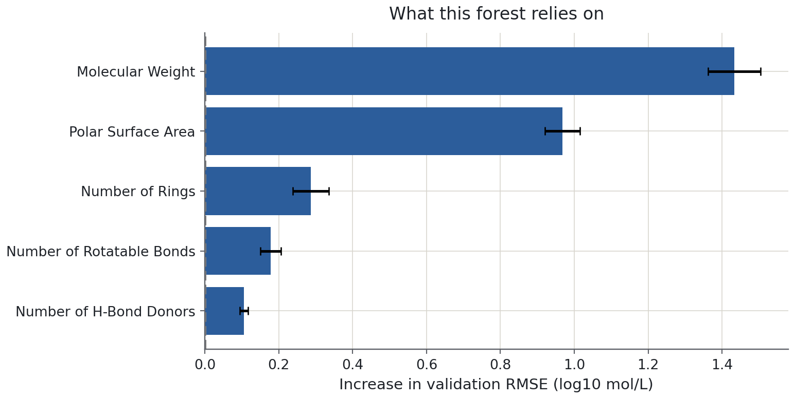
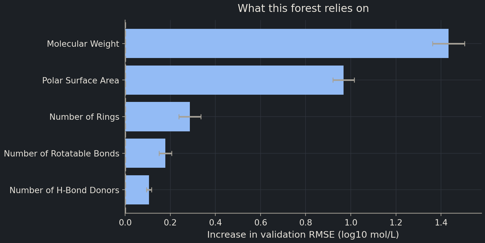
permutation importance asks how much predictive score deteriorates when a feature column is shuffled across evaluation rows. The shuffle preserves its observed values but breaks their alignment with the other features and targets. If the model relies on that feature for useful prediction, the score should worsen.

Repeat the shuffle to see how sensitive the result is to that random perturbation. With scoring="neg_root_mean_squared_error", an importance is the original negative-RMSE score minus the shuffled score. A positive value therefore means an increase in RMSE after shuffling, in logS units. This sign is easy to misread.

Predict before you run

If two descriptors contain nearly the same information, must each have high permutation importance? Think about what the model can still use when just one is shuffled.

from sklearn.inspection import permutation_importance

permutation = permutation_importance(
    model, X_valid, y_valid, scoring="neg_root_mean_squared_error",
    n_repeats=15, random_state=42, n_jobs=1
)
importance = pd.DataFrame({"feature": features,
                           "RMSE increase": permutation.importances_mean,
                           "shuffle SD": permutation.importances_std})
importance.sort_values("RMSE increase", ascending=False).round(3)

index	feature	RMSE increase	shuffle SD
0	Molecular Weight	1.433	0.071
4	Polar Surface Area	0.967	0.047
2	Number of Rings	0.287	0.048
3	Number of Rotatable Bonds	0.178	0.028
1	Number of H-Bond Donors	0.106	0.011

import matplotlib.pyplot as plt

ordered = importance.sort_values("RMSE increase")
fig, ax = plt.subplots(figsize=(8, 4))
ax.barh(ordered["feature"], ordered["RMSE increase"],
        xerr=ordered["shuffle SD"], capsize=3)
ax.axvline(0, color="0.5", linestyle="--")
ax.set(xlabel="Increase in validation RMSE (log10 mol/L)",
       title="What this forest relies on")
plt.show()

Permutation importance for five solubility descriptors, shown as the increase in validation RMSE after each column is shuffled. Error bars show variation across shuffles, not a confidence interval.

A feature near zero may be unused, redundant with others, or too weakly measured to demonstrate an effect here. A slightly negative value can occur when shuffling happens to improve predictions; it is not evidence that the descriptor physically decreases solubility. The error bars describe repeated shuffling of one fixed validation set, not uncertainty over new datasets or refitted models.

Correlated features complicate interpretation: the model may substitute one for another, or the shuffle may create unrealistic combinations. Tree impurity-based importance has additional biases, including favouring features with many possible split values. Permutation importance on held-out data asks a more directly predictive question, but still depends on the evaluation distribution and metric. See the permutation-importance guide for these distinctions.

Chemist's corner

Shuffling polar surface area while leaving molecular weight and donor count fixed can describe combinations that no real molecule in this collection has. The experiment perturbs a table column, not a chemical structure. A large score change tells you that the model uses that association; it does not tell you how to synthesise a more soluble compound.

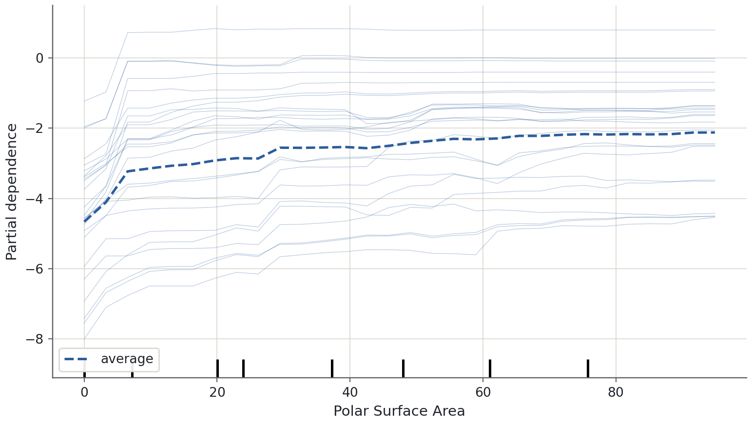
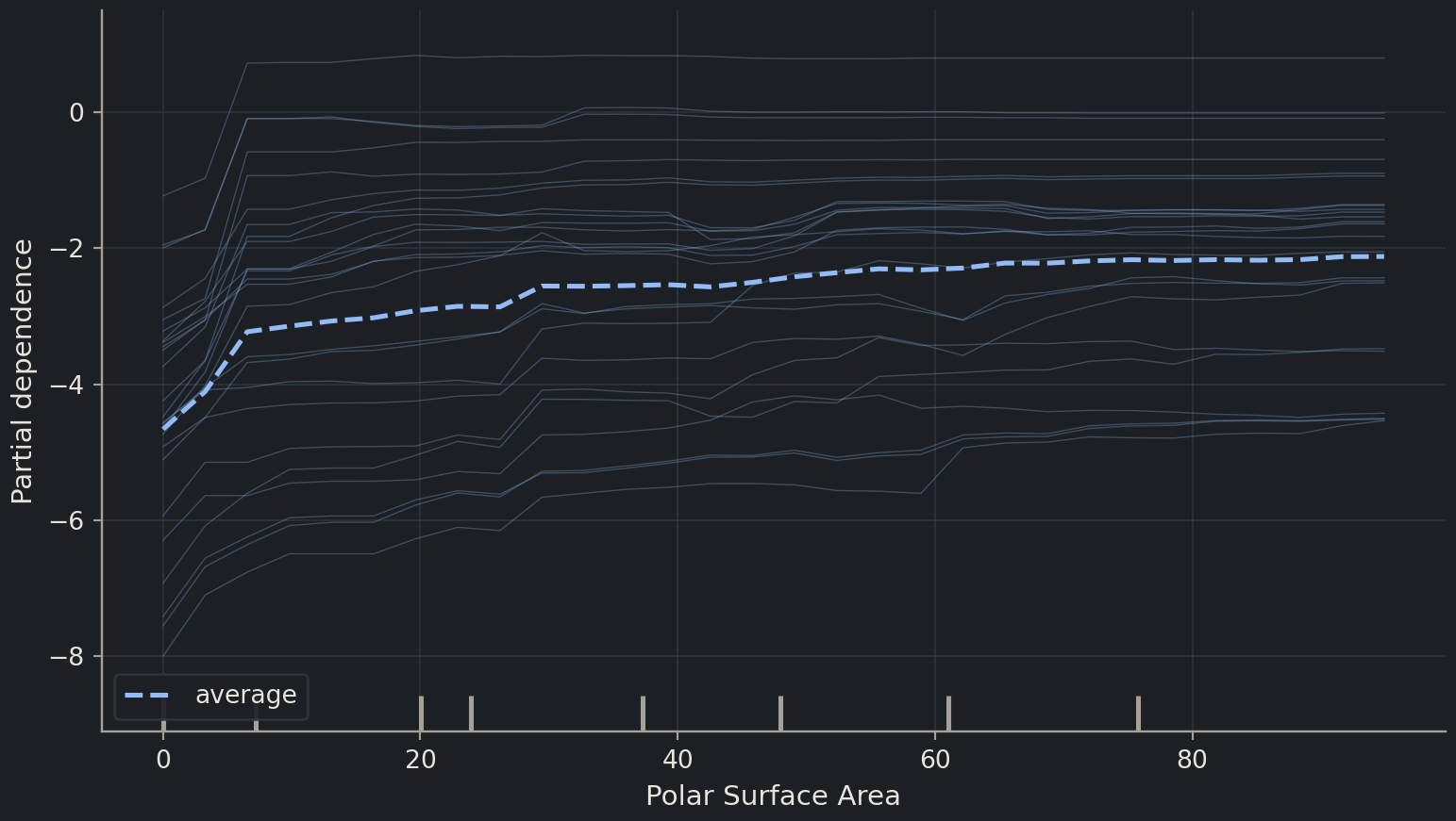
Partial dependence averages hypothetical responses

For a chosen feature value, replace that feature in every evaluation row, predict, and average the predictions. Repeating over a grid gives partial dependence. It summarises the fitted model’s average response over the other features represented in the selected table.

An individual conditional expectation (ICE) curve keeps the response of one row instead of averaging. Several ICE curves can reveal interactions that the average conceals: increasing a descriptor may change predictions differently for different backgrounds. These are model responses to hypothetical table edits, not observed experimental dose–response curves. The partial-dependence documentation explains the connection between individual and average curves.

from sklearn.inspection import PartialDependenceDisplay

fig, ax = plt.subplots(figsize=(8, 4.5))
PartialDependenceDisplay.from_estimator(
    model, X_valid, features=["Polar Surface Area"], kind="both",
    subsample=25, random_state=42, grid_resolution=30,
    method="brute", ax=ax
)
ax.set(xlabel="Polar surface area (angstrom squared)",
       ylabel="Model response (log10 mol/L)")
plt.show()

Partial dependence and a sample of individual conditional expectation curves for polar surface area. Thin curves show how individual validation-row predictions respond to hypothetical changes; the bold curve shows the average model response.

Read the horizontal range before interpreting the trend. The displayed grid focuses on the observed feature distribution; it is not a licence to extrapolate outside it. The small marks along the axis indicate the distribution of observed values. Sparse regions provide less direct support for the hypothetical combinations.

Parallel ICE curves suggest a similar response across these backgrounds, while differing slopes or step locations suggest interactions. A flat partial-dependence curve could hide strong opposing effects that cancel in the mean. When features are tightly correlated, both PDP and ICE may traverse implausible combinations, so inspect relationships in the original data alongside the curves.

Local explanations answer a different question

Global importance summarises dependence across a dataset. A local attribution instead describes one prediction relative to a reference. A common additive form is

\[f(x) = \phi_0 + \sum_j \phi_j,\]

where \(\phi_0\) is a reference prediction and \(\phi_j\) is an attributed contribution for feature \(j\). SHAP-style methods use a Shapley-value allocation derived from a specified feature-coalition game. The background data, treatment of missing features and treatment of feature dependence influence the explanation; the contributions are not uniquely determined by the prediction alone. This is a conceptual preview, and no extra explanation library is needed for the lab.

An additive explanation can say “relative to this background, these descriptor values contributed to the model’s low prediction”. It cannot establish “changing this one molecular property will change measured solubility by this contribution”. Changing a real structure may alter many descriptors, move outside the reference distribution and invoke mechanisms absent from the fitted model.

Inspect where the errors occur

A global importance ranking can look sensible while hiding a region where predictions fail. Before proposing a chemical explanation, compare errors across a small set of scientifically motivated groups. Define the groups using the fitting data or external knowledge, not by repeatedly cutting validation rows until an interesting contrast appears. Here we use molecular-weight quartiles from the fitting partition, extending the edge bins to cover all validation rows.

boundaries = np.r_[-np.inf, X_fit["Molecular Weight"].quantile([0.25, 0.5, 0.75]), np.inf]
residual = y_valid - model.predict(X_valid)
diagnostics = pd.DataFrame({
    "size group": pd.cut(X_valid["Molecular Weight"], boundaries),
    "absolute error": residual.abs(), "squared error": residual ** 2,
})
group_errors = diagnostics.groupby("size group", observed=True).agg(
    samples=("absolute error", "size"), MAE=("absolute error", "mean"),
    MSE=("squared error", "mean"))
group_errors["RMSE"] = np.sqrt(group_errors.pop("MSE"))
group_errors.round(3)

index	samples	MAE	RMSE
size group	index	index	index
(-inf, 119.126]	47	0.509	0.705
(119.126, 182.154]	63	0.484	0.643
(182.154, 275.613]	60	0.727	1.038
(275.613, inf]	56	0.740	1.031

Read the sample counts with the errors. A group containing few observations can show an extreme average because of one bad prediction. The grouping also does not isolate molecular size as a cause: size may track ring count, measurement conditions or other unmeasured properties. A useful report identifies a performance limitation without claiming that the grouping variable explains it.

If the largest-size group has worse errors, the next step might be checking which molecules and conditions it contains, then testing whether the same pattern appears in another development fold. If all groups look similar, that rules out only this coarse diagnostic; it does not prove uniform performance for every chemical subgroup. Predeclared group analyses reduce the temptation to tell a story around whichever partition happens to look striking.

The same habit transfers to patients, assay batches or sequence families. Report both aggregate performance and relevant subgroup behaviour, while protecting enough data for the final independent assessment. Inspection should sharpen a testable question, not turn exploratory differences into unsupported mechanisms.

Turn an explanation into a testable hypothesis

Use interpretation to choose the next investigation, not to end it. If errors are large for very polar molecules, inspect measurement conditions and which structural information the descriptor table omits. If one apparent driver is a proxy for collection batch, examine whether performance survives a batch split. If importance rankings fluctuate across folds, report that instability instead of presenting one confident ordering.

For correlated descriptors, a grouped permutation can shuffle related columns together, preserving their internal relationships while breaking their association with the remaining table. It answers a group-level reliance question, not the unique effect of each feature. Choose groups from scientific knowledge or development-data analysis, and keep the eventual test independent of those choices.

Common mistake

Inspection can become hidden model selection

Removing a descriptor because it has low test-set importance is a model change informed by the test set. The revised model needs new independent evaluation. Development-fold explanations are the appropriate place to explore feature removal; final test explanations may accompany a frozen result but must not be used to retain the same untouched-test claim after revision.

Exercises

Exercise★☆☆

Interpret the sign and units

The original validation RMSE is 0.8. After shuffling a feature it averages 1.1. What permutation importance is reported with the negative-RMSE scorer, and what does it mean?

SolutionShow solution

The importance is \((−0.8)−(−1.1)=+0.3\) logS units. Shuffling that feature increased this fitted model’s validation RMSE by 0.3 on average. It is neither a regression coefficient nor the change in measured solubility caused by changing the feature.

Exercise★★☆

Test a grouped reliance question

Shuffle donor count and polar surface area together using the same row permutation. Compare the resulting RMSE with the original. Why use one shared permutation?

SolutionShow solution

rng = np.random.default_rng(42)
columns = ["Number of H-Bond Donors", "Polar Surface Area"]
shuffled = X_valid.copy()
order = rng.permutation(len(X_valid))
shuffled.loc[:, columns] = X_valid.iloc[order][columns].to_numpy()
original_error = root_mean_squared_error(y_valid, model.predict(X_valid))
group_error = root_mean_squared_error(y_valid, model.predict(shuffled))
print(f"Grouped shuffle RMSE increase: {group_error - original_error:.3f}")

Grouped shuffle RMSE increase: 0.997

One permutation preserves each observed donor-count/area pair. It breaks that pair’s relation to the other columns and target. This one shuffle is only a demonstration; repeated shuffles and repeated fitting partitions are needed to assess different sources of variability.

Exercise★★★

Rewrite a causal claim

Rewrite “polar surface area is the cause of solubility because it has the highest importance” as a defensible finding and a separate follow-up hypothesis.

SolutionShow solution

Finding: “For this fitted model and validation set, disrupting polar surface area produced the largest measured score decrease among the tested descriptors.” Hypothesis: “Polar interactions or correlated structural properties may help explain solubility variation; test this in a designed series with controlled measurement conditions.” The first reports model behaviour; the second proposes an investigation rather than claiming its result.

Where this is going

The chapter lab combines honest selection with a development-data interpretation and a final frozen test evaluation. Chapter 4 adds neural networks, whose extra flexibility makes these boundaries even more valuable. Model explanations are useful scientific tools when their claims stay within the evidence that produced them.

Key points

Check predictive quality before interpreting a fitted model’s behaviour.
Permutation importance measures a score drop for a particular model, dataset and metric.
Correlated features can share importance and make hypothetical feature changes unrealistic.
Partial dependence averages model responses; ICE reveals variation across individual rows.
Explanations describe model behaviour and do not establish an intervention’s causal effect.