How can a model learn interactions without a formula for each one?
Why does a tree that fits perfectly often predict poorly?
What you will be able to do
Read the decisions and predictions of a shallow regression tree.
Choose tree complexity using training-only cross-validation.
Explain why a tree can be unstable and cannot extrapolate a trend.
A large molecule can still dissolve well if it has suitable polar groups. The effect of size can depend on the rest of the structure: one global slope for molecular weight may be too restrictive. A decision treedecision treeA model that follows feature-threshold questions to a terminal region and its prediction. learns a sequence of questions such as “is the polar surface area below this threshold?” and follows a different prediction rule down each branch. It captures an interaction when a later question depends on an earlier answer.
That flexibility comes with a cost. With enough questions, a tree can create a tiny region around almost every training molecule. Its predictions then record the observations rather than a pattern that survives in new data. We will make the questions visible and use cross-validationcross-validationEvaluating a fitting procedure over multiple training and held-out subsets chosen to match the prediction task. to decide how many are useful.
The data and the evaluation boundary
Keep the descriptor table and target from Chapter 2. One row represents a molecule; logS is measured in log₁₀(mol/L). We reserve the same test rows for the eventual project, but do not use their scores in this lesson.
from pathlib import Pathimport numpy as npimport pandas as pdurl ="https://deepchemdata.s3-us-west-1.amazonaws.com/datasets/delaney-processed.csv"path = Path("data/esol.csv")esol = pd.read_csv(path if path.exists() else url)features = ["Molecular Weight", "Number of H-Bond Donors", "Number of Rings","Number of Rotatable Bonds", "Polar Surface Area"]X = esol[features]y = esol["measured log solubility in mols per litre"]X.shape, y.shape
((1128, 5), (1128,))
from sklearn.model_selection import KFold, train_test_splitX_train, X_test, y_train, y_test = train_test_split( X, y, test_size=0.2, random_state=42)cv = KFold(n_splits=5, shuffle=True, random_state=42)print(f"Development rows: {len(X_train)}; reserved test rows: {len(X_test)}")
Development rows: 902; reserved test rows: 226
The split boundary is part of the experiment. A tree’s ability to overfit does not justify a more forgiving test protocol. Nor does a nonlinear algorithm repair duplicate molecules, related measurements in both sets, or a descriptor calculated using the target. Those problems occur before model fitting.
A prediction is the mean in a leaf
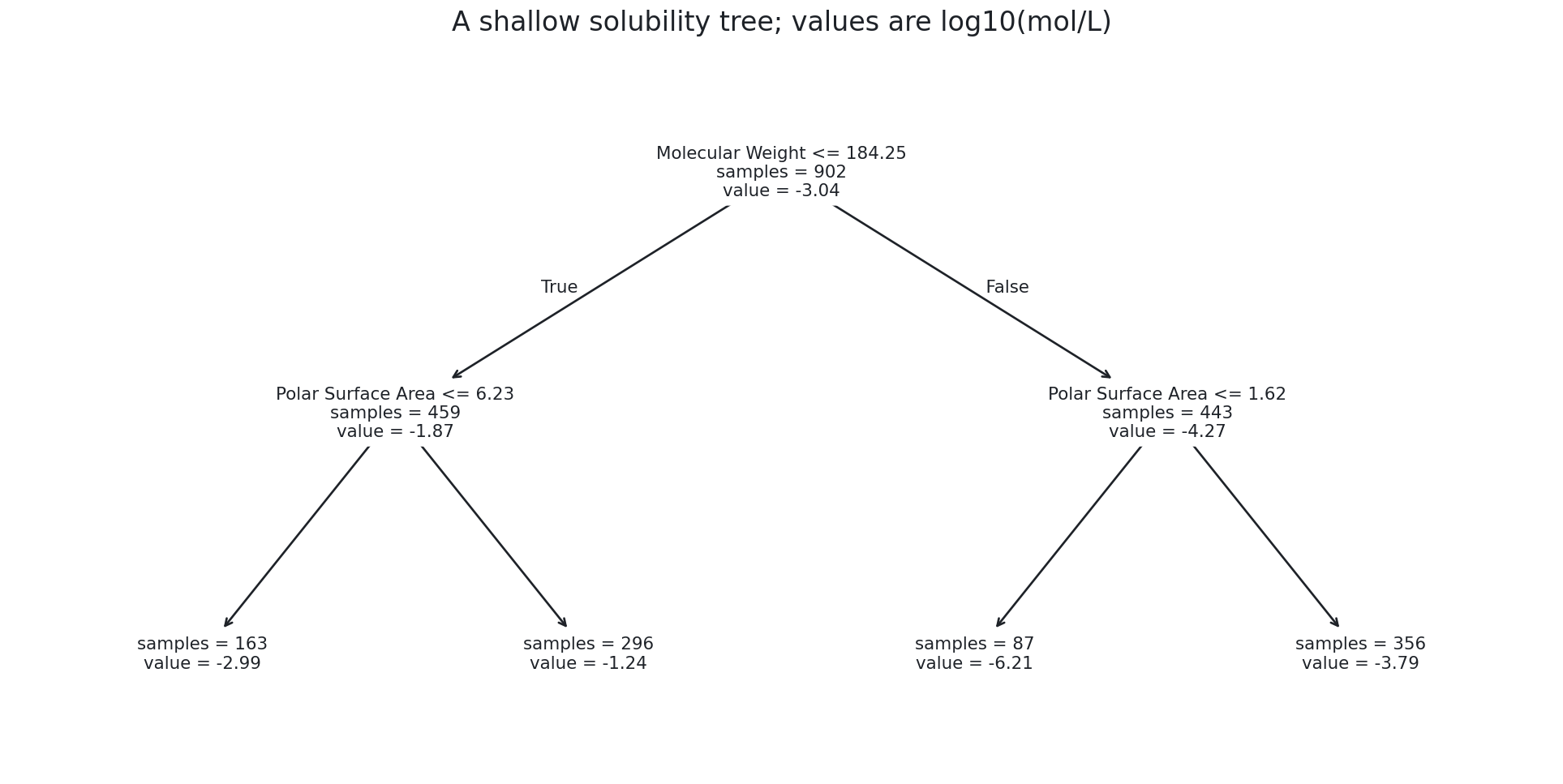
Imagine dividing the training table into two groups according to molecular weight. For each group, predict its mean measured logS. A candidate division is good if those two means leave less squared error than predicting one mean for everyone. The algorithm tries feature thresholds and chooses the largest available reduction, then repeats within each child group.
With the default squared-error criterion, a regression leaf predicts the mean of the training targets assigned to it. A classifier instead estimates class proportions in its leaves and predicts a class from them. Thus a tree applies the same partitioning idea to two different learning tasks; regression values and class probabilities are not interchangeable outputs.
Read the output from the top. Follow the <= or > branch at every question; the final value is the predicted logS. A depth of two allows at most four leaves. Different paths can ask about different features, so the resulting rule is already more flexible than one line through all molecules.
Chemist's corner
Think of a tree as a decision key used at the bench: first ask one question, then choose the next question from the answer. Unlike a mechanistic decision key, these cut-offs were selected to reduce error in a particular dataset. A split at one precise molecular weight does not imply a physical discontinuity in solubility at that value.
The sample counts make the evidence behind each prediction visible. A prediction supported by 300 observations and one supported by 3 observations deserve different levels of trust, even if their values look equally precise. Leaf counts are a useful diagnostic, though they are not prediction intervals: a large leaf can still mix chemically different molecules and miss systematic effects.
Trees compare ordered thresholds, so changing grams to milligrams preserves the order and usually the same partitions, apart from numerical effects. Standardisation is therefore unnecessary for this estimator. Scaling can still be present in a shared comparison pipeline, but it does not give a tree the benefits it gives a distance-based method.
Common mistake
A rule is not a mechanism
If the tree asks about rings before polar surface area, that does not show that rings cause solubility changes or are universally more important. Correlated descriptors may substitute for each other. Inspecting a different training sample may give a different first question with similar predictive performance.
Tune complexity without opening the test set
Three useful controls are max_depth, the longest path; min_samples_leaf, the smallest supported terminal group; and ccp_alpha, the strength of cost-complexity pruning. Pruning removes branches whose improvement is too small relative to the added complexity. Start with a small, scientifically reasonable search rather than tuning every knob at once. The scikit-learn tree guide documents these controls and the estimator’s limitations.
Predict before you run
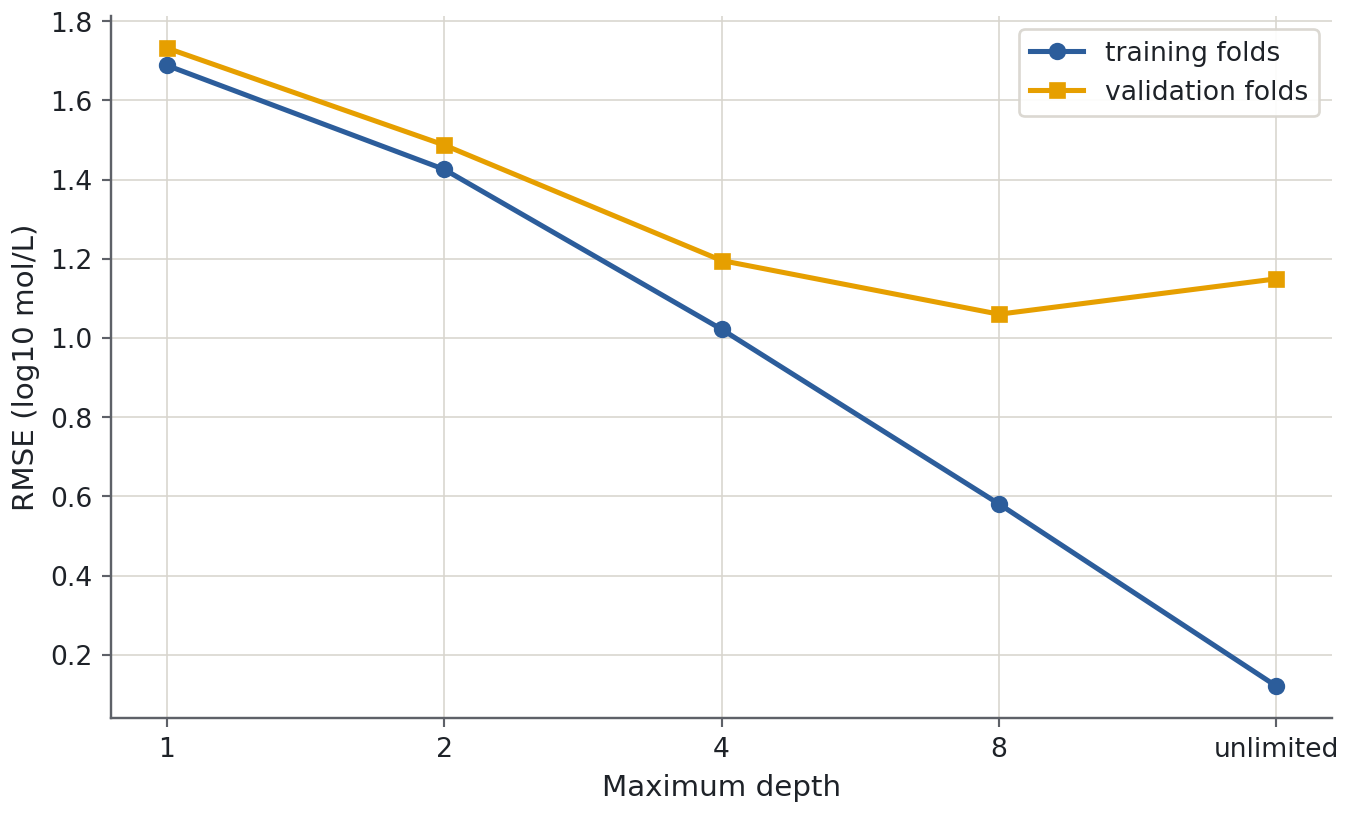
What will happen to training RMSE as depth increases? Will validation RMSE necessarily follow it? Predict the two curves before running the experiment.
test_score is scikit-learn’s name for the held-out fold score; here it is a development validation score, not a result on X_test. Negating the scores restores RMSE in logS units. A fall in training error with a flat or rising validation error tells you that extra branches are fitting details that do not transfer between folds.
The lowest row is a candidate setting, not proof of its final performance. We have just selected among five depths using these folds, so the minimum CV error is mildly optimistic for the chosen setting. A reserved test set or outer CV loop estimates the full selection procedure. If two depths are very close, favouring the shallower one can make predictions easier to inspect, provided that preference is stated before the final evaluation.
Classification changes the leaf summary
For a toxicity flag, the questions still divide observations, but squared-error reduction is no longer the usual split criterion. A classifier can prefer splits that make the class proportions more concentrated. One measure is Gini impurity, \(1-\sum_c p_c^2\), where \(p_c\) is the fraction of training observations of class \(c\) in a node. A node containing only one class has zero impurity; a balanced binary node has impurity 0.5.
Consider a node with ten positive and ten negative examples. A split into two equally sized children, one with nine positives and one with nine negatives, makes each child less mixed. A split that merely puts five positives and five negatives in each child changes the sample count but does not improve class separation. The algorithm scores a candidate using the sample-weighted impurity of both children, so an excellent tiny child does not automatically justify a poor large one.
At a terminal leaf, the training class proportions supply the classifier’s probability estimate. A leaf with one positive example can therefore output probability 1, even though its empirical support is only one observation. Requiring larger leaves may reduce such extremes, but it does not guarantee calibration. Check probability quality separately on appropriate held-out data if decisions depend on risk estimates.
This also explains why the fitting criterion and evaluation metric need not be identical. A classifier might fit using Gini impurity, choose complexity using balanced accuracy, and ultimately support an action whose threshold reflects false-negative and false-positive costs. Declare those roles separately. No change of split criterion removes the need for a relevant baseline, an appropriate positive-class definition and independent evaluation.
What a tree cannot do
A regression tree predicts one of its leaf means, so its predictions stay within the training target range. If the data contain only small molecules, asking about an enormous new molecule will send it into an existing leaf. The tree does not continue a size–solubility trend beyond the observed domain. Random forests inherit this averaging limitation, while boosted trees have a different additive construction but still should not be trusted to extrapolate an unseen physical trend.
Instability is another limitation. A small change in data may make a different split win near the root, changing every later branch. A fixed random seed makes one fitting run reproducible; it does not make the learned rule robust to new samples. To assess robustness, repeat a predeclared evaluation or inspect fits on resampled development data. Never choose the seed that produces the best score.
Discussion
Two depth-two trees achieve similar validation errors but ask different first questions. What could you report confidently, and what claim about the chemistry would be unsupported? Distinguish predictive stability from stability of the explanation.
Exercises
Exercise★☆☆
A leaf by hand
A terminal region contains three training logS values: −2, −3 and −7. What does a squared-error regression tree predict for a new molecule in that region? What information is hidden by that prediction?
SolutionShow solutionHide solution
It predicts the mean, −4 log₁₀(mol/L). That single number hides a five-log-unit range and the possibility that the leaf mixes different chemical regimes. Adding another justified split may help; reporting the mean alone does not establish certainty.
Exercise★★☆
Require more evidence per leaf
Compare min_samples_leaf values 1, 5 and 20 at max_depth=8, using the same folds. Which result would support increasing the leaf size?
Support comes from lower development validation error or similar error with a simpler, more stable rule. A higher training error is expected and is not, on its own, a reason to reject the larger leaf size.
Exercise★★☆
Debug this: the persuasive tree
Someone fits 50 depths and selects whichever has the lowest RMSE on X_test. They publish the selected tree’s test RMSE and its diagram as evidence of a chemical law. Identify two distinct problems.
SolutionShow solutionHide solution
The test rows have become a validation set through repeated selection; use training-only CV for depth and evaluate once on genuinely untouched data. Separately, the diagram describes associations learned by one model. Even an honestly evaluated tree does not establish that changing a descriptor would cause the predicted chemical change.
Where this is going
The next episode combines many trees to reduce the instability of one fit or to correct errors sequentially. Later, molecular fingerprints will give trees thousands of structural questions to ask. The same discipline remains: control complexity, choose a split that matches the intended new molecules, and keep the final test outside all decisions.
Key points
A tree partitions feature space with successive questions and predicts a constant within each leaf.
Depth, leaf size and pruning control complexity; select them without consulting the final test set.
A readable decision rule describes a fitted model, not a causal law.
Trees need no standardisation but still require honest splitting and sensible features.