How can similarity produce a nonlinear prediction?
What do C and gamma control, and why does scaling matter?
What you will be able to do
Explain a maximum-margin classifier and an epsilon-insensitive regressor.
Tune a scaled support vector regression pipeline on development folds.
Read a two-parameter validation surface without using the test set.
If two molecules have similar descriptor values, should their solubilities be similar? Often enough to be useful, but not always: a small structural change can matter greatly. A support vector machine turns a chosen notion of similarity into a prediction rule. Its usefulness therefore depends both on how it learns and on whether the descriptors preserve the distinctions the scientific question needs.
We will first build intuition using classification, then fit support vector regression to ESOL. The distinction matters: a separating boundary and a numeric prediction are different outputs, even though both use support vectors and can share the same kernel.
A margin is room around a boundary
For two classes, many boundaries may separate the training examples. A linear support vector classifier prefers a boundary with a wide marginmarginThe separation between a decision boundary and nearby supporting observations.: distance between the separating hyperplane and the nearest supporting observations. With noisy or overlapping classes, insisting on perfect separation can produce an unhelpful boundary. A soft margin permits violations and balances them against the width of the margin.
The parameter C sets the penalty for those violations. A larger C makes violations more costly and can encourage a more intricate fit when a nonlinear kernel is used. A smaller C tolerates more violations in exchange for stronger regularisation. Notice the direction: increasing C generally weakens regularisation, whereas increasing ridge’s alpha strengthens it. Their numerical values are not comparable.
The support vectors are training observations that determine the fitted boundary through the optimisation. They are not a hand-picked representative subset or necessarily the most biologically important samples. An outlier or an ambiguous measurement can become a support vector precisely because it is difficult to fit.
Biologist's corner
Imagine separating two populations of measured cells by a gate. A comfortable gap makes the separation less sensitive to small measurement changes. An SVM formalises a related preference, but optimises in the chosen feature space. If a batch effect creates the gap, a wide margin can still be scientifically misleading.
A kernel replaces explicit feature expansion
A linear boundary may be inadequate. One way to obtain a curved boundary is to construct extra features such as squared measurements and products, then fit a linear model in that expanded space. A kernelkernel functionA similarity function used to build a predictor in an implicit feature space. computes the relevant similarity between examples without requiring us to write down every expanded coordinate.
The radial basis function, or RBF, kernel uses squared Euclidean distance:
Nearby observations have similarity close to one; distant observations have similarity close to zero. A large gamma makes that similarity fall rapidly, allowing local variation. A small gamma spreads influence over a wider region. This explains why C and gamma should be considered together. The official RBF parameter example illustrates these two controls.
Common mistake
A numerical distance has scientific assumptions
Without scaling, molecular weight values in the hundreds can dominate donor counts of only a few units. Standardisation changes the geometry by putting each feature on a comparable scale. It does not prove that one standard deviation in molecular weight is chemically equivalent to one standard deviation in polar surface area; it is a modelling choice to test.
Regression uses a tolerance tube
Support vector regression (SVR) predicts a continuous target. Its epsilon-insensitive loss assigns no fitting penalty to errors within a tube of width epsilon on either side of the predicted value. Outside that tube, the penalty grows with the excess error. C again controls the cost of violations, while gamma controls locality for the RBF kernel.
For our unscaled target, epsilon=0.1 means a tolerance of 0.1 logS units, not 0.1 mol/L. The tube is part of the fitting objective; it is not a prediction interval and does not give a probability that future measurements fall inside it. Changing target units changes the sensible epsilon and C ranges.
Prepare a leak-free pipeline
from pathlib import Pathimport numpy as npimport pandas as pdfrom sklearn.model_selection import KFold, train_test_spliturl ="https://deepchemdata.s3-us-west-1.amazonaws.com/datasets/delaney-processed.csv"path = Path("data/esol.csv")esol = pd.read_csv(path if path.exists() else url)features = ["Molecular Weight", "Number of H-Bond Donors", "Number of Rings","Number of Rotatable Bonds", "Polar Surface Area"]X = esol[features]y = esol["measured log solubility in mols per litre"]X_train, X_test, y_train, y_test = train_test_split( X, y, test_size=0.2, random_state=42)cv = KFold(n_splits=5, shuffle=True, random_state=42)X_train.shape
The scaler learns means and standard deviations when fit runs. When the pipeline is passed to a search, each fold receives a fresh scaler fitted to its training rows. The corresponding validation rows are transformed using those training statistics. Scaling the complete development table first would leak validation information even though the final test set remained untouched.
Search a small, logarithmic grid
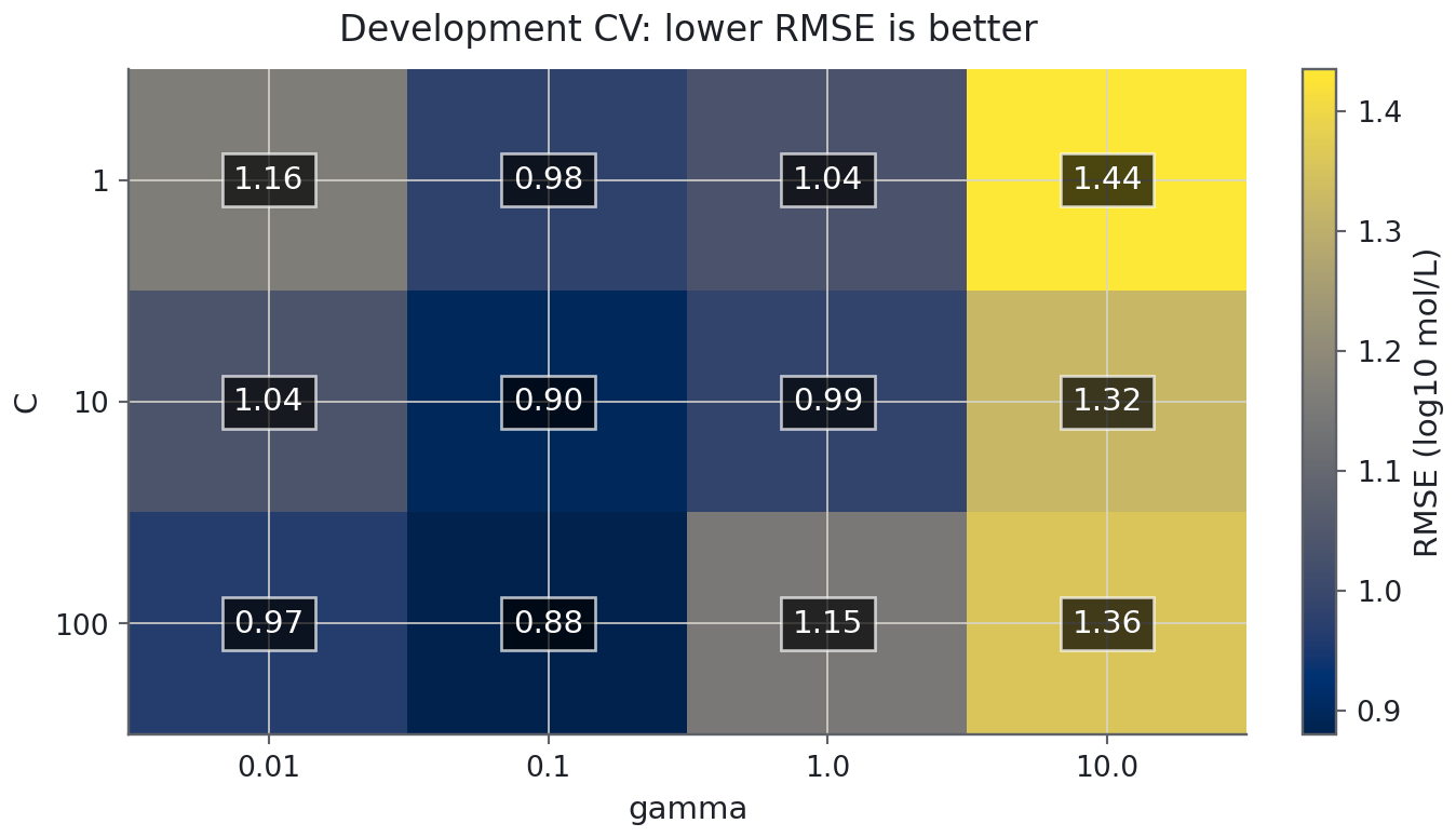
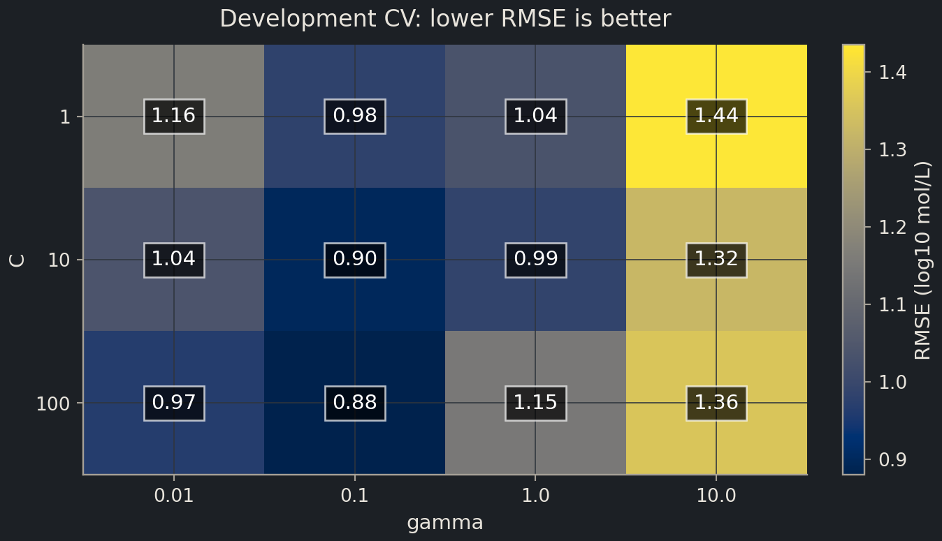
Try settings across orders of magnitude. Values such as C=1, 10, 100 test meaningfully different penalty strengths; adding C=10.1 before understanding the broad range wastes the search budget. This first search contains 12 configurations and five folds, so it performs 60 CV fits plus one refit of the chosen configuration on the complete development set.
Predict before you run
Which combination is most likely to be very local and flexible: small C with small gamma, or large C with large gamma? Will the most flexible combination necessarily have the lowest validation RMSE?
{'svr__C': 100, 'svr__gamma': 0.1}
Selected development CV RMSE: 0.880
best_estimator_ is a complete fitted pipeline. Its scaler is refitted on all development rows, and the SVR is trained in that resulting coordinate system. Keep them together for later predictions. Saving the regressor alone would lose the transformation that gives its distances meaning.
A broad region of similar errors is often more reassuring than one isolated winning cell. It suggests the result is less sensitive to precise settings. A winner at the edge may motivate extending the range on development data, but this makes the search adaptive and uses more validation evidence. Document that choice; do not inspect the final test to decide which direction to extend.
Compare SVR with the nearest-neighbour intuition
Both k-nearest neighbours and an RBF SVR depend on distances, but they do not use neighbours in the same way. kNN identifies the closest training rows at prediction time and averages their targets, optionally using distance weights. Its main locality control is how many neighbours contribute. SVR instead learns coefficients during a global optimisation; support vectors contribute to the fitted prediction through kernel similarities, and those contributions need not form a simple positive average of nearby targets.
The loss also differs. For a regression residual \(e=y-f(x)\), epsilon-insensitive loss is \(\max(0, |e|-\epsilon)\). If epsilon is 0.1 and the absolute residual is 0.06 logS units, this part of the fitting loss is zero. An absolute residual of 0.4 contributes 0.3. Errors within the tolerance still contribute to evaluation RMSE: ignoring them in the optimisation does not erase them from the scientific assessment.
An experiment might motivate epsilon from a rough measurement-resolution scale, but it is not automatically an estimate of measurement noise. Replicate assays, laboratory effects and censored solubility values could complicate that relationship. Select a defensible range using development evidence and document the interpretation; do not infer an assay’s precision from whichever epsilon minimises a tuning score.
This comparison suggests a useful diagnostic before celebrating a gain. If both kNN and SVR improve dramatically on a random split but fail when related molecules are kept together, the problem may be that nearby training analogues made the task unusually easy. Changing the algorithm does not change the intended generalisation question. Compare them under the same representation and chemically appropriate split before attributing a benefit to the kernel method itself.
Costs, probabilities and extrapolation
Kernel SVMs can become costly as the number of samples grows because they work with pairwise relationships. A dataset with about a thousand rows is a useful setting for this experiment. With very large tables, consider a linear method or an approximation, and evaluate runtime as well as predictive error. Feature count, sample count and support-vector count all affect practical cost.
For classification, SVC.decision_function returns a signed score, not a probability. probability=True enables an additional probability-estimation procedure, with additional fitting cost; probability quality still requires assessment on held-out data. A well-ranked classifier can be poorly calibrated. The threshold for an action should reflect its costs and be selected using development data, as in Chapter 2.
For an RBF model far from all training observations, the kernel similarities approach zero. Its behaviour there should not be interpreted as a learned physical trend. Neither a smooth surface nor a confident class label establishes that a new molecule lies within the model’s useful domain. In molecular work, chemical similarity and applicability checks will matter alongside numeric descriptor distance.
Exercises
Exercise★☆☆
Reverse the regularisation knob
Someone says “ridge alpha and SVM C are both regularisation strengths, so increasing either makes the fit simpler.” Correct the statement.
SolutionShow solutionHide solution
Increasing ridge alpha strengthens its coefficient penalty. Increasing SVM C strengthens the penalty for fitting violations, generally allowing a less regularised fit. Their directions differ, and neither parameter has a transferable numerical scale between models or datasets.
Exercise★★☆
Inspect the support vectors
Find how many training rows became support vectors in the selected SVR. Why does a high proportion matter when predicting many new molecules?
SolutionShow solutionHide solution
fitted_svr = search.best_estimator_.named_steps["svr"]n_support =int(fitted_svr.n_support_.sum())print(f"Support vectors: {n_support} of {len(X_train)} training rows")
Support vectors: 791 of 902 training rows
Prediction uses kernel comparisons with the support vectors, so a high count can increase prediction cost and storage. It does not by itself show overfitting or poor quality; judge generalisation separately with the declared evaluation.
Exercise★★★
A physically impossible neighbour
Two molecules have almost identical values for all five descriptors yet different measured logS. Can increasing gamma guarantee a solution? Suggest a better investigation.
SolutionShow solutionHide solution
No. Identical feature vectors cannot be distinguished by this deterministic model, and near-identical inputs may reflect measurement noise or missing structural information. Check measurement conditions and duplicates, then consider structural features such as fingerprints. Evaluate the revised representation inside the selection procedure; do not add features after seeing the test errors and retain the old test claim.
Where this is going
The next episode asks what the descriptor geometry looks like before predicting a target. In Part II, molecular fingerprints introduce a different representation and similarity measure. The lesson transfers: a kernel’s mathematical convenience does not replace scientific reasoning about what “similar” should mean.
Key points
A kernel expresses similarity; the RBF kernel makes nearby feature vectors influence each other more strongly.
Scale features inside every training fold before fitting a distance-based kernel model.
C controls the penalty for errors; gamma controls the locality of the RBF similarity.
An SVM decision score is not automatically a calibrated probability.