Build a multilayer perceptron and count its trainable parameters.
Explain why nonlinear activation functions are needed between linear layers.
Match regression and classification targets to compatible outputs and losses.
Molecular mass and polarity can interact: a change in one descriptor need not have the same effect everywhere in chemical space. A linear model uses one coefficient per feature across the entire dataset. A neural network learns intermediate features and combines them, allowing more flexible relationships. Whether that flexibility helps must still be tested against the classical baselines from Chapters 2 and 3.
A multilayer perceptron (MLP)multilayer perceptron (MLP)A feedforward neural network that alternates learned linear maps with nonlinear activations., or multilayer perceptron, is a useful first network for a table of numerical descriptors. Its layers are arranged in sequence, and each sample passes through the same sequence. It provides the core mechanics of deep learning without requiring images, sequences or a GPU.
Hidden layers are learned feature transformations
For an input matrix \(X\), one hidden layer computes \(H=\phi(XW_1+b_1)\), then the output layer computes \(z=HW_2+b_2\). The weights and biases are learned parameters. The activation functionactivation functionA usually nonlinear transformation applied to a layer’s values, such as ReLU or tanh.\(\phi\) acts elementwise and makes the transformation nonlinear. The number of columns in \(H\), called the hidden width, is a hyperparameter.
The word hidden means these intermediate features are neither the supplied descriptors nor the target. It does not mean they are inaccessible: you can inspect their values. Their units and meanings are generally not the original physical units, and assigning a chemical interpretation to a hidden unit requires evidence beyond looking at one weight.
This model maps five descriptors to 16 hidden features, applies a rectified linear unit, then maps those features to one output. nn.Sequential passes the output of each module into the next. The weights are initialised by the layers; they are not all zero. The four zero rows above are a shape check, not a useful dataset for training.
The PyTorch Linear documentation defines the layer’s affine transformation and parameter shapes. Its weight array is stored as (out_features, in_features), so a manual reconstruction uses X @ layer.weight.T + layer.bias. That storage convention differs from the mathematical \(W\) written above, while the transformation is the same.
Predict before you run
Count the trainable numbers in this network before running the next cell. Remember that each output of a linear layer has one bias. Does the ReLU add any trainable parameters?
for name, parameter in model.named_parameters():print(name, tuple(parameter.shape), parameter.numel())print("total parameters:", sum(p.numel() for p in model.parameters()))
The first layer has \(5\times16+16=96\) parameters; the output layer has \(16\times1+1=17\), for a total of 113. ReLU has none. Increasing width from 16 to 160 increases the number of learned parameters even if the number of training examples stays fixed. Parameter count is a useful capacity check, although it alone does not determine generalisation.
Why the activation matters
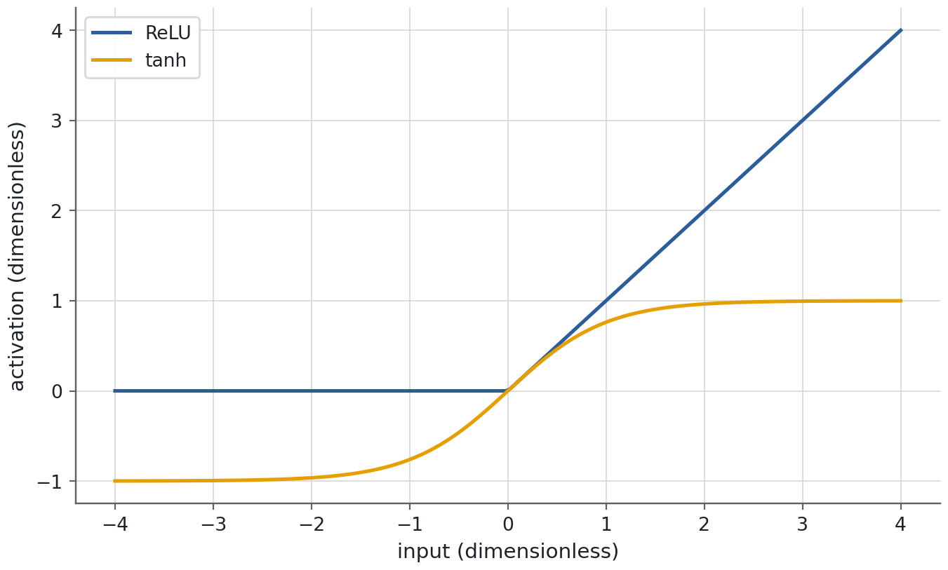
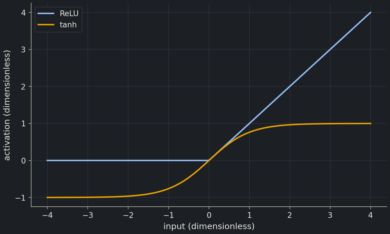
ReLU applies \(\max(0,z)\) to each value. Negative inputs become zero and positive inputs pass through unchanged. As the input changes, different hidden units become active, allowing the network to represent a piecewise linear function. Smooth activations such as Tanh are alternatives, but their different gradients and ranges change optimisation.
Without the activation, two affine layers collapse into one: \((XW_1+b_1)W_2+b_2=X(W_1W_2)+(b_1W_2+b_2)\). Adding another linear layer would add parameters and alter the optimisation problem, but it would not make the represented function nonlinear. The activation is therefore part of the model’s expressive capacity, not merely a decorative layer between matrix multiplications.
Biologist's corner
An intermediate feature can combine several measured quantities, much as a summary score combines several assay readouts. The network learns these combinations to improve its prediction objective. That does not make a hidden unit a discovered pathway, cell type or causal mechanism. A useful predictive representation and a validated biological explanation are different scientific claims.
Common mistake
A unit can stop contributing
A ReLU with negative input for every training example produces zero output and zero local gradient through that activation. Poor scaling or overly large updates can make learning harder. Start with standardised features, modest widths and a sensible learning rate; inspect training and validation curves before adding more layers.
Choose the output from the target
Architecture should finish with an output that matches the question. For one continuous logS target, use one unrestricted real output and an appropriate regression loss such as MSE. A sigmoid would constrain predictions to zero through one, which is incompatible with negative logS values unless you had deliberately transformed the target and documented the inverse transform.
For binary classification, one real output can be a logitlogitA real-valued classification score supplied before a sigmoid or softmax probability transformation.: a score that becomes a probability through the sigmoid. For mutually exclusive multiclass classification, produce one real score per class. The loss then compares those scores with the observed class.
Task
Model output
Target
Training loss
One continuous property
(n,), unrestricted real values
(n,), floating point
MSELoss
One binary label
(n,), raw logits
(n,), floating-point 0 or 1
BCEWithLogitsLoss
One of C classes
(n, C), raw logits
(n,), integer class indices
CrossEntropyLoss
These are defaults for the tasks shown, not a list of all possible losses. Multilabel classification, where several labels can be present simultaneously, differs from mutually exclusive multiclass classification. Likewise, changing a regression target to a logarithmic scale changes what MSE penalises; specify the target’s scale in the report.
Suppose an educational classifier labels three samples as 0, 1 and 1. A logit of zero corresponds to probability 0.5. Positive logits favour class 1; negative logits favour class 0. Very confident incorrect predictions should incur a large penalty, so the training loss uses the scores, not the hard class decisions.
BCEWithLogitsLoss combines the sigmoid and binary cross-entropy in a numerically stable implementation. Pass it raw logits; do not add a sigmoid layer first. Apply the sigmoid afterwards when reporting probabilities or using a chosen decision threshold. This input contract is documented in BCEWithLogitsLoss.
The loss is a smooth objective for fitting. Accuracy, recall and ROC AUC answer different evaluation questions. A threshold can be chosen on validation data to reflect the intended costs, then fixed before test evaluation. A sigmoid output is not automatically a well-calibrated probability: calibration needs its own held-out assessment.
Multiclass classification and regression
For three mutually exclusive classes, use three logits and a single integer target per sample. The target says which column is correct; it is not a floating-point measurement and does not need one-hot encoding for this common CrossEntropyLoss interface.
Softmax normalises across the class axis so each sample’s probabilities sum to one. Do not normalise across the sample axis: that would make one sample’s prediction depend on what other samples happen to be in its batch. As with the binary loss, supply raw logits to the training loss and transform them only when needed for interpretation.
For regression, match prediction and target shapes and retain the units. If you standardise the target using training statistics, optimise in that standardised space and invert the transformation before reporting MAE or RMSE. Otherwise a dimensionless loss may be mistaken for an error in log₁₀(mol/L).
A small network is useful because you can inspect its inputs, parameter count and training behaviour. Begin with one hidden layer, then add complexity only in response to validation evidence. More width, more layers, a different activation and dropout are all hyperparameters; changing them repeatedly after looking at test results is test leakage.
For a small descriptor table, ridge, logistic regression, random forests or boosting may be competitive or better. A network earns its place through an honest comparison with the same examples and metric. In later chapters its main advantage may come from learning representations of graphs or sequences, rather than simply applying more parameters to five fixed descriptors.
Exercises
Exercise★☆☆
Count before you train
A network maps 30 inputs to 12 hidden units, then to one binary logit. It uses a ReLU between the two linear layers. How many trainable parameters does it have?
SolutionShow solutionHide solution
The first layer has \(30\times12+12=372\) parameters. The second has \(12+1=13\). ReLU has no trainable parameters, so the total is 385. The number of samples in a batch does not change this total: every sample uses the same weights.
Exercise★★☆
Repair the output contract
Three networks finish with a sigmoid: one predicts logS, one uses BCEWithLogitsLoss for a binary target, and one uses CrossEntropyLoss for four mutually exclusive classes. Explain the correction for each.
SolutionShow solutionHide solution
The logS model needs an unrestricted scalar output with a regression loss. The binary model needs one raw logit for BCEWithLogitsLoss; use sigmoid only for reporting. The four-class model needs four raw logits for CrossEntropyLoss, with a one-dimensional integer target; use softmax across classes for reporting. Loss and output must be designed together.
Exercise★★★
A nonlinear network that acts linearly
Can a ReLU network still behave like a linear model over the range of inputs you observed? Explain why fitting a neural network does not by itself demonstrate a nonlinear scientific relationship.
SolutionShow solutionHide solution
Yes. If the pattern of active ReLUs stays fixed over that range, the composition within it is affine. A trained network may also approximate a line even when activation patterns differ. Compare its validated performance and predicted response shapes against a linear baseline, accounting for uncertainty and confounding. The architecture’s capacity is not evidence that the underlying relationship requires that capacity.
Where this is going
Episode 4.4 trains a complete classifier in mini-batches and separates training from evaluation. In Chapter 7, a graph model will replace the fixed descriptor input with learned atom and bond representations. The final output and loss will still be chosen from the prediction target using the same contracts.
Key points
A multilayer perceptron alternates learned linear maps with nonlinear activations.
Stacking linear layers without nonlinearities still represents an affine function.
Use raw logits with BCEWithLogitsLoss or CrossEntropyLoss; apply probability transforms for reporting.
Network capacity is a modelling choice, not evidence of better generalisation.