4.5 Validation, regularisation and honest comparison

45 min of teaching25 min of exercisesintermediate

Questions this episode answers

How do I stop at the best epoch without touching the test set?
When should I prefer a simpler model to a neural network?

What you will be able to do

Restore a copied checkpoint selected by validation loss.
Distinguish dropout, weight decay and early stopping.
Compare a network with a classical baseline under the same evaluation protocol.

A flexible network can continue reducing training loss after its validation performance stops improving. The practical question is no longer whether the code can fit the observations; it is which fitted model you should keep and how much evidence supports it. More computation does not automatically answer that question.

Three controls are useful: early stopping limits training using validation evidence, dropout randomly disables some activations during training, and weight decay shrinks parameters during optimisation. Each changes the fitted model, so its settings are hyperparameters. None repairs a leaking split or replaces a comparison against a simpler method.

Keep one experiment’s data boundaries

We reproduce the previous episode’s split so this page runs independently. The validation subset chooses the epoch. The test subset remains unopened until a later, final evaluation. In a larger project, store the split indices rather than relying on remembering a seed and the order of the data file.

import torch
from sklearn.datasets import load_breast_cancer
from sklearn.model_selection import train_test_split
from sklearn.preprocessing import StandardScaler

data = load_breast_cancer(as_frame=True)
X, y = data.data, (data.target == 0).astype(int)
X_dev, X_test, y_dev, y_test = train_test_split(
    X, y, test_size=0.2, stratify=y, random_state=42)
X_train, X_val, y_train, y_val = train_test_split(
    X_dev, y_dev, test_size=0.25, stratify=y_dev, random_state=42)
scaler = StandardScaler().fit(X_train)
Xtr = torch.tensor(scaler.transform(X_train), dtype=torch.float32)
Xva = torch.tensor(scaler.transform(X_val), dtype=torch.float32)
ytr = torch.tensor(y_train.to_numpy(), dtype=torch.float32)
yva = torch.tensor(y_val.to_numpy(), dtype=torch.float32)
print("training / validation:", len(ytr), len(yva))

training / validation: 341 114

The scaler is fitted on X_train, not X_dev: validation has already been removed. In cross-validation, this entire operation must happen inside each training fold. Creating a scaler once outside the fold loop would leak information, even if a newly initialised network were fitted inside each fold.

Dropout and weight decay

Dropout sets a random fraction of activations to zero during training and rescales the retained values. It discourages the network from relying on one particular set of active units. At evaluation, the standard module stops dropping values. The Dropout documentation specifies this train/evaluation behaviour.

Weight decay in AdamW is decoupled from its adaptive gradient update. Do not assume that adding an L2 term to the loss has exactly the same effect for every optimiser. Here the parameter-shrinkage strength is explicit in the optimiser configuration, and our starting value is a demonstration to assess, not a recommendation for all datasets. See AdamW for its update rule.

from torch import nn

torch.manual_seed(42)
model = nn.Sequential(
    nn.Linear(Xtr.shape[1], 16), nn.ReLU(), nn.Dropout(p=0.1), nn.Linear(16, 1))
loss_fn = nn.BCEWithLogitsLoss()
optimiser = torch.optim.AdamW(model.parameters(), lr=0.003, weight_decay=0.01)
print(model)

Sequential(
  (0): Linear(in_features=30, out_features=16, bias=True)
  (1): ReLU()
  (2): Dropout(p=0.1, inplace=False)
  (3): Linear(in_features=16, out_features=1, bias=True)
)

Predict before you run

Call a dropout layer twice on the same input in training mode, then twice in evaluation mode. In which mode can the outputs differ? Would repeatedly evaluating the test set until one random output looks good be a valid comparison?

dropout = nn.Dropout(p=0.5)
ones = torch.ones(8)
dropout.train()
print("training:", dropout(ones), dropout(ones))
dropout.eval()
print("evaluation:", dropout(ones), dropout(ones))

training: tensor([0., 0., 2., 0., 0., 0., 0., 0.]) tensor([0., 2., 0., 0., 2., 2., 0., 0.])
evaluation: tensor([1., 1., 1., 1., 1., 1., 1., 1.]) tensor([1., 1., 1., 1., 1., 1., 1., 1.])

In training mode the outputs can differ because the masks are sampled randomly. In evaluation mode this standalone layer returns its input unchanged. Selecting a favourable test result among repeated runs would bias the estimate; the selection procedure is part of what must be evaluated honestly.

Chemist's corner

Early stopping resembles choosing a reaction time using a development experiment, then applying the chosen protocol to an independent batch. Looking at the independent batch after every time point and choosing the best result would turn it into another optimisation experiment. Dropout and weight decay are additional modelling controls, not evidence that a model has learned chemically valid rules.

Save the best weights, not a reference to changing weights

Early stopping needs four decisions: the monitored metric, the minimum improvement, the number of non-improving epochs allowed (patience), and a maximum epoch budget. Validation loss is convenient because it is smooth and matches this training objective. If your selection target is another metric, specify it before comparing candidates and use its correct direction.

from torch.utils.data import DataLoader, TensorDataset

loader = DataLoader(TensorDataset(Xtr, ytr), batch_size=32, shuffle=True,
                    generator=torch.Generator().manual_seed(42))
def train_epoch():
    model.train()
    for features, targets in loader:
        optimiser.zero_grad(set_to_none=True)
        loss = loss_fn(model(features).squeeze(1), targets)
        loss.backward()
        optimiser.step()

print("mini-batches per epoch:", len(loader))

mini-batches per epoch: 11

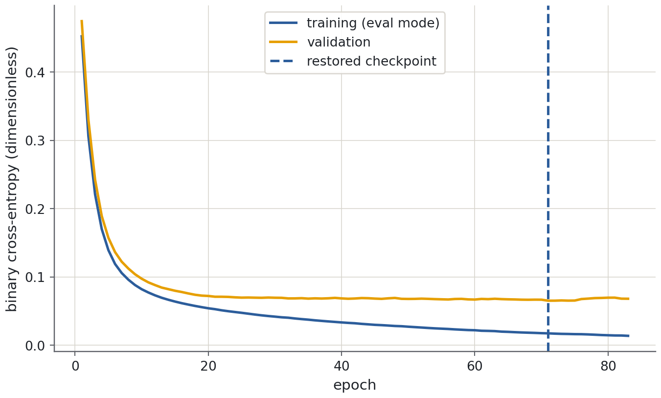
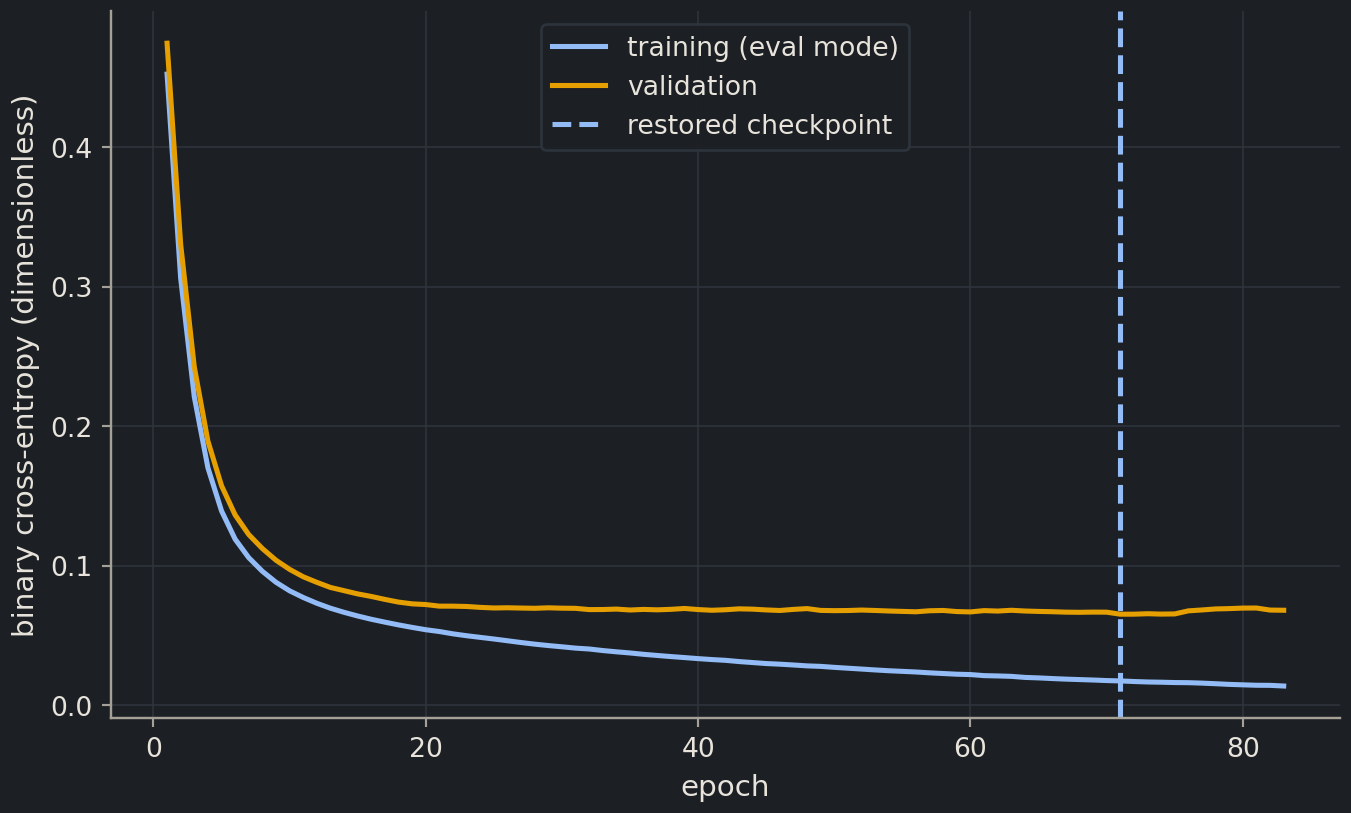
The training function performs only updates on training data. The following evaluator computes losses for the final weights of the epoch with dropout disabled. That makes the two curves comparable; otherwise the training curve would include the extra perturbation from dropout while the validation curve would not.

def loss_on(features, targets):
    model.eval()
    with torch.no_grad():
        return loss_fn(model(features).squeeze(1), targets).item()

print("initial validation loss:", loss_on(Xva, yva))

initial validation loss: 0.6768267154693604

A state_dict maps parameter names to tensors. To preserve the best epoch in memory, make an independent copy. A plain best_state = model.state_dict() can retain references whose contents change as training continues, so it may fail to preserve the model you intended. The PyTorch saving guide explicitly describes this checkpointing issue.

from copy import deepcopy

best_loss, best_epoch, stale = float("inf"), 0, 0
patience, min_delta = 12, 1e-4
history = []
for epoch in range(1, 151):
    train_epoch()
    train_loss, val_loss = loss_on(Xtr, ytr), loss_on(Xva, yva)
    history.append((train_loss, val_loss))
    if val_loss < best_loss - min_delta:
        best_loss, best_epoch, stale = val_loss, epoch, 0
        best_state = deepcopy(model.state_dict())
    else:
        stale += 1
    if stale >= patience:
        break
model.load_state_dict(best_state)
print("epochs run / chosen epoch:", len(history), best_epoch)
print("restored validation loss:", loss_on(Xva, yva))

epochs run / chosen epoch: 83 71
restored validation loss: 0.06521143019199371

The selected epoch may precede the final epoch run. Restoring its weights is essential; stopping and keeping the last model would implement a different procedure. min_delta prevents tiny changes from resetting patience. Because of that tolerance, the chosen checkpoint is the last sufficiently improved value, not necessarily the mathematical minimum of every recorded float.

import numpy as np
import matplotlib.pyplot as plt

curves = np.asarray(history)
fig, ax = plt.subplots()
ax.plot(np.arange(1, len(curves) + 1), curves[:, 0], label="training (eval mode)")
ax.plot(np.arange(1, len(curves) + 1), curves[:, 1], label="validation")
ax.axvline(best_epoch, linestyle="--", label="restored checkpoint")
ax.set(xlabel="epoch", ylabel="binary cross-entropy (dimensionless)")
ax.legend()
plt.show()

Training and validation cross-entropy over epochs with a vertical line at the selected checkpoint, which can occur before training stops.

Compare with an explicit baseline

A neural network’s training curve can look impressive while a simpler model performs equally well. Fit a fixed logistic-regression pipeline on the same training rows and compare both methods using validation log loss. This is a development comparison; its winning score is optimistic for the choice it helped make, and it must not be labelled test performance.

from sklearn.pipeline import make_pipeline
from sklearn.linear_model import LogisticRegression
from sklearn.metrics import log_loss
import pandas as pd

baseline = make_pipeline(StandardScaler(), LogisticRegression(C=1.0, max_iter=2000))
baseline.fit(X_train, y_train)
baseline_loss = log_loss(y_val, baseline.predict_proba(X_val))
comparison = pd.Series({"logistic regression": baseline_loss,
                        "early-stopped MLP": loss_on(Xva, yva)}, name="validation log loss")
print(comparison.round(4))

logistic regression    0.0717
early-stopped MLP      0.0652
Name: validation log loss, dtype: float64

Read the displayed ordering rather than assuming the network wins. If their performance is close, computation, ease of debugging, reproducibility and interpretation can favour logistic regression. A larger network is not a stronger baseline merely because it has more parameters.

For a fairer tuned comparison, give each model a declared search budget. Logistic regression’s C and the network’s width, learning rate, dropout and decay all need training-only selection. A single validation set may be practical for an expensive model, while cross-validation or nested CV is useful when data are small and the budget permits. Whichever design you choose, compare on identical held-out observations and retain the complete selection history.

Reproducibility is more than one seed

Save the split identifiers, feature order, fitted scaler, architecture, state dictionary, hyperparameters, chosen epoch and package versions. To resume training exactly, also save optimiser state and the relevant random-generator states. Loading a state dictionary into a matching architecture is a different operation from recreating the complete training experiment.

A fixed seed helps repeat a run in a given environment. It does not guarantee identical outputs across devices, versions or every operation; see PyTorch reproducibility notes. Report the software and device along with the seed. When comparing models, inspect several prespecified seeds on development data and report variability instead of selecting the luckiest run.

Common mistake

The validation set can also be overused

Trying hundreds of architectures, patience values and seeds against one small validation set can fit its noise. Keep the search budget bounded, record the comparisons and use an independent outer evaluation when assessing a selection procedure. The standard deviation across training seeds describes initialisation sensitivity; it is not a confidence interval for performance on a new population.

From development to final evaluation

After choosing the model family and settings, state how the final model will be fitted before opening the test set. One valid option is to retain the training-only model selected with validation. Another is to refit preprocessing and a fresh model on all development data for a fixed epoch count chosen earlier. Do not use the test set for early stopping during that refit.

The lab uses the first option so every step remains visible. It chooses between a ridge baseline and a small network for ESOL on validation performance, then reports their prespecified final test comparison without revising the choice. Random molecular splits remain a teaching convenience: near-duplicate chemistry and extrapolation to new scaffolds need the more demanding experiments developed in Part II.

Exercises

Exercise★☆☆

Which weights belong in the report?

The lowest sufficiently improved validation loss occurs at epoch 24, patience expires at epoch 36, and training loss is lowest at epoch 36. Which weights should an early-stopped model use, and why?

SolutionShow solution

Use the saved epoch-24 weights. The procedure selects according to validation performance, so the extra epochs only establish that a new qualifying improvement did not appear within patience. Keeping epoch 36 would discard the stated selection rule. Report both the selected epoch and the total training budget when useful.

Exercise★★☆

A misleading checkpoint

A colleague uses best_state = model.state_dict() after each improvement and later calls load_state_dict(best_state). Why might this fail to restore the best model? Give the in-memory correction and name two non-weight objects needed for future predictions.

SolutionShow solution

The dictionary’s tensors can refer to values updated by subsequent training. Save deepcopy(model.state_dict()) to preserve independent values. Future predictions also require the matching architecture and preprocessing contract, including the fitted scaler and feature order. Weights alone do not describe how raw scientific measurements become model inputs.

Exercise★★★

A fair comparison with a budget

You have time for 12 network fits and one fixed test set. Propose a small search and explain how you would treat random seeds and early stopping without consulting the test labels.

SolutionShow solution

One option is four prespecified combinations of width and learning rate, each run with three prespecified seeds on the same training/validation split. Fix dropout, decay, patience and the maximum epoch budget initially. Compare mean validation performance and variability, choose a declared final-run policy, then evaluate the frozen procedure on the test set. For stronger evidence on a small dataset, allocate a larger budget to nested or repeated outer splits rather than interpreting the best of 12 validation scores as an unbiased estimate.

Where this is going

Lab 4 brings the entire workflow back to molecular solubility: tensors, mini-batches, early stopping, classical baselines and a final test report. You are then ready for Part II, where the main new question is how to represent a molecule and evaluate transfer to unfamiliar chemistry. The honest-evaluation habits remain the foundation even when the model architecture changes.

Key points

Early stopping chooses an epoch using validation data and must restore its saved weights.
Dropout changes training behaviour; evaluation disables it.
AdamW weight decay is a separate parameter-shrinkage operation.
Seeds support repeatability; several seeds and honest splits assess robustness.
A final test result estimates a frozen procedure and must not select its settings.