3.5 Clustering: useful groups without supplied labels
35 min of teaching20 min of exercisesintermediate
Questions this episode answers
What does it mean for unlabelled samples to form a group?
How can I assess clusters when I do not know the correct answer?
What you will be able to do
Fit k-means to scaled measurements and inspect cluster profiles.
Interpret inertia, silhouette and a hierarchical dendrogram.
Check clustering stability and distinguish clusters from biological classes.
Suppose a field team returns with bill measurements, flipper lengths and body masses but has not recorded species. Can the measurements reveal useful groups? clusteringclusteringGrouping observations by a chosen representation and similarity rule without supplied target labels. searches for structure without supplied target labels. It can organise observations for inspection or suggest hypotheses, but it cannot certify that a group is a species, a cell type or a molecular mechanism.
We return to the penguins from Chapter 1. We will deliberately exclude the species column while constructing clusters and inspect it only afterwards as external context. In a genuinely unlabelled dataset that comparison would be unavailable; the geometry and the experimental metadata would have to carry more of the argument.
Decide what “nearby” should mean
Two penguins can be similar in bill dimensions but different in body mass. A distance calculation requires a choice about how those measurements count. Using raw values would make grams dominate millimetres numerically. Standardising each feature gives a change of one training standard deviation comparable numerical weight across measurements.
That is a transparent default, not a universal biological truth. Repeating a correlated measurement in ten columns would also give its underlying variation more influence. Feature selection and transformations therefore help define the clusters; they are not neutral housekeeping done before the “real” algorithm.
from pathlib import Pathimport numpy as npimport pandas as pdfrom sklearn.preprocessing import StandardScalerpenguins = pd.read_csv(Path("data/penguins.csv"))features = ["bill_length_mm", "bill_depth_mm", "flipper_length_mm", "body_mass_g"]observed = penguins.dropna(subset=features).copy()X = observed[features]scaler = StandardScaler()Z = scaler.fit_transform(X)print(f"Complete rows: {len(X)}; excluded for missing measurements: {len(penguins) -len(X)}")
Complete rows: 342; excluded for missing measurements: 2
We use complete cases for a compact exploratory demonstration and report what was excluded. In a research analysis, missingness could be systematic: for example, harder-to-handle animals might lack a measurement. Compare missingness across known groups before assuming the remaining sample represents the population. An imputation procedure would be another modelling choice to document.
K-means alternates assignments and centres
k-meansk-meansA clustering algorithm that minimises squared distances to k cluster centres. starts with \(k\) centres, assigns each observation to its closest centre, moves each centre to the mean of its assigned observations, and repeats. Its objective is the sum of squared distances from observations to their assigned centres. This quantity is called inertia in scikit-learn.
The algorithm can settle at different local solutions depending on its initial centres. n_init=10 runs ten initialisations and retains the one with lowest inertia. A fixed random_state makes this procedure reproducible. It does not prove that the chosen groups are robust to new observations or another plausible distance metric.
Predict before you run
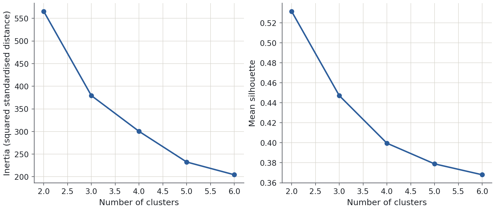
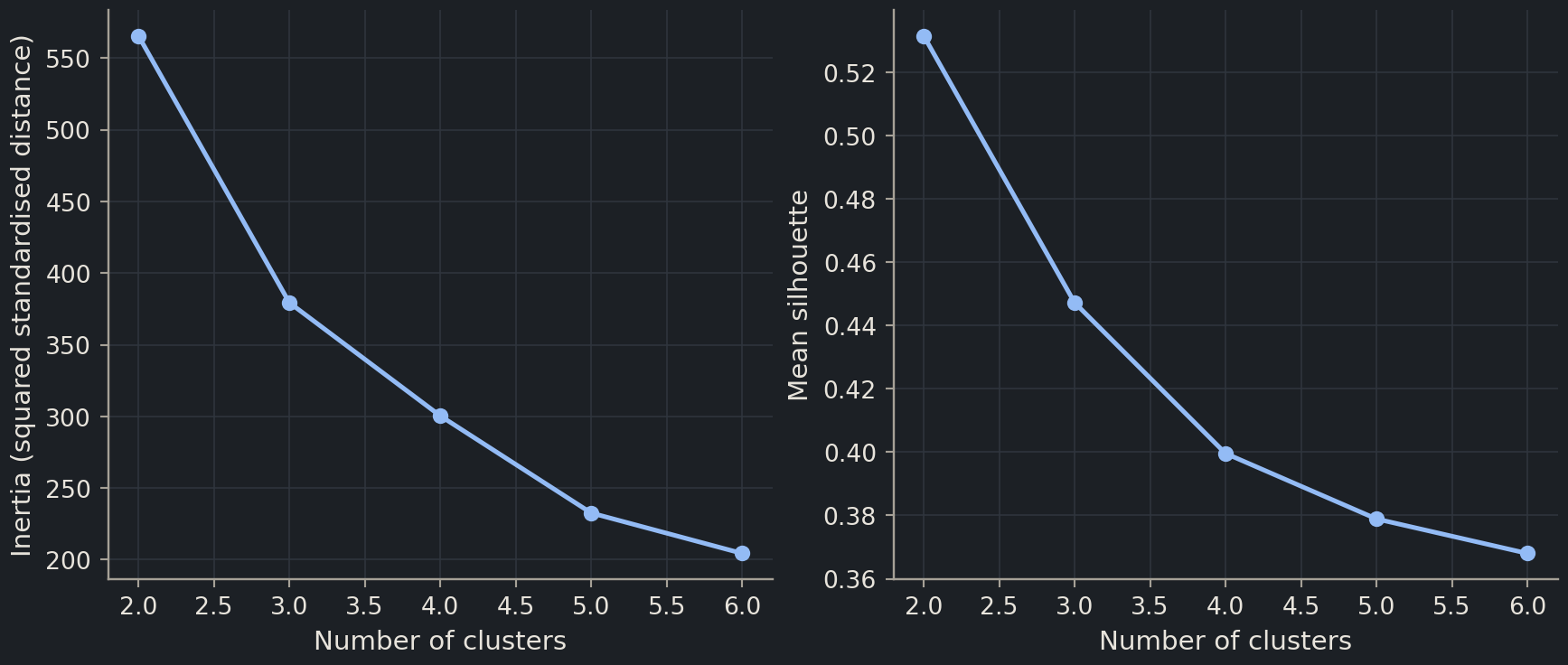
If we increase k from 2 to 6, can the best achievable training inertia increase? Does lower inertia alone tell us which k is scientifically best?
from sklearn.cluster import KMeansfrom sklearn.metrics import silhouette_scorerows = []for k inrange(2, 7): model = KMeans(n_clusters=k, n_init=10, random_state=42).fit(Z) rows.append({"k": k, "inertia": model.inertia_,"silhouette": silhouette_score(Z, model.labels_)})diagnostics = pd.DataFrame(rows)diagnostics.round(3)
index
k
inertia
silhouette
0
2
565.708
0.532
1
3
379.393
0.447
2
4
300.400
0.400
3
5
232.605
0.379
4
6
204.393
0.368
More centres can make regions smaller and reduce the best possible inertia, even when the extra divisions have no scientific value. In practice local optimisation can produce imperfect solutions, which is one reason to use several initialisations. The “elbow” heuristic looks for diminishing returns in inertia, but an elbow may be absent or ambiguous.
Read silhouette as a geometric diagnostic
The silhouette coefficientsilhouette coefficientA geometric measure comparing within-cluster distance with distance to the nearest other cluster. of a sample compares its average distance to its own cluster with the average distance to the nearest other cluster. Values near 1 suggest a well-separated assignment, near 0 a boundary point, and negative values a point closer on average to another group. The score depends on the distance and representation, and favours some cluster shapes over others. The clustering guide describes the assumptions and evaluation measures.
import matplotlib.pyplot as pltfig, axes = plt.subplots(1, 2, figsize=(9, 3.8))axes[0].plot(diagnostics["k"], diagnostics["inertia"], "o-")axes[0].set(xlabel="Number of clusters", ylabel="Inertia (squared standardised distance)")axes[1].plot(diagnostics["k"], diagnostics["silhouette"], "o-")axes[1].set(xlabel="Number of clusters", ylabel="Mean silhouette")plt.show()
Use these summaries to identify plausible descriptions, then inspect the groups. A silhouette score cannot say whether a split reflects species, sex, island, age or a measurement artefact. Selecting the largest score produces the best value among the settings tried; it does not establish a unique natural partition.
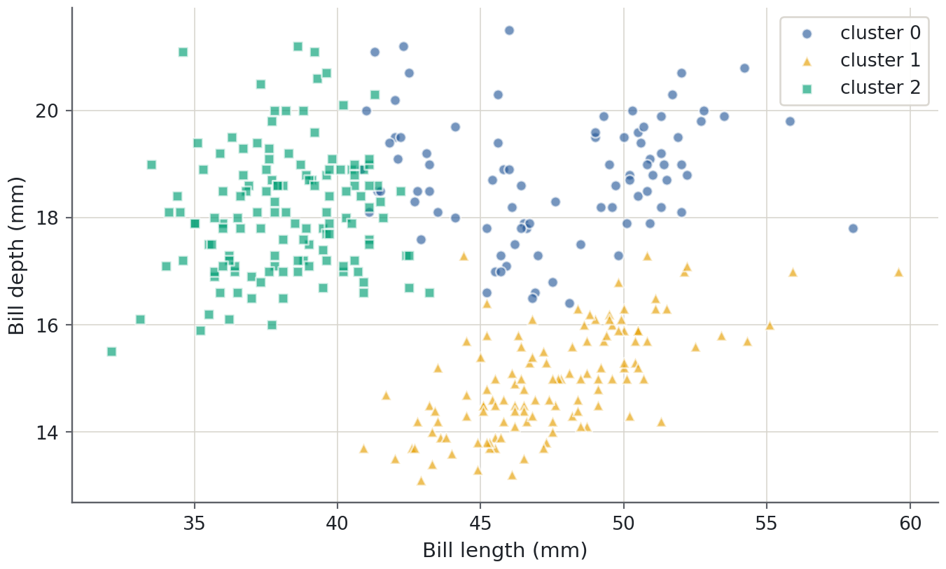
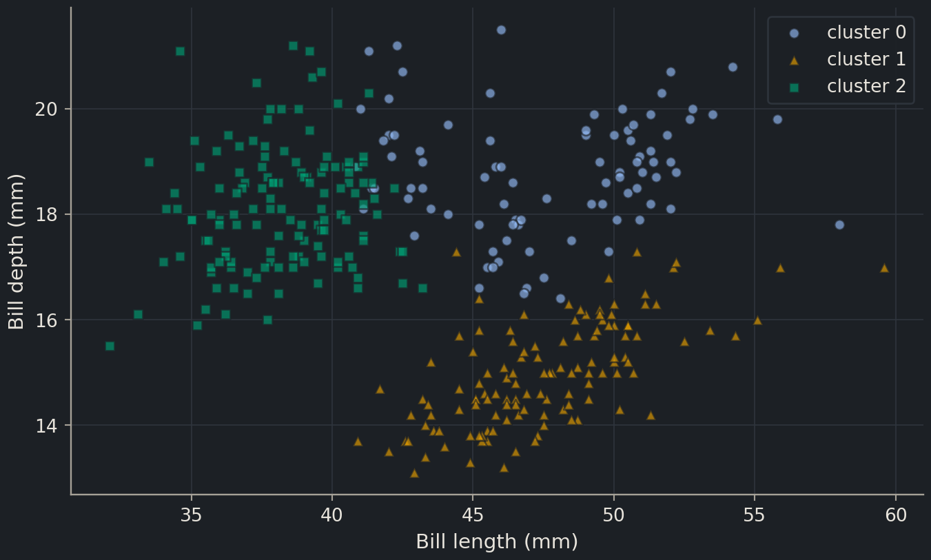
For interpretation we now choose three clusters as a declared teaching example, not because we claim that a diagnostic proved three is correct. Keep that distinction explicit: a demonstration of an algorithm should not be disguised as a discovery.
These means are back in familiar units because we grouped the original measurements. Give the clusters provisional descriptions such as “larger average body mass” rather than naming them as species immediately. Also inspect cluster sizes and within-group variation: a mean can hide a broad or multimodal group.
Biologist's corner
In single-cell data, a cluster might reflect a cell type, cell-cycle phase, donor, sequencing depth or an injured-cell state. Assigning a biological name requires marker evidence and experimental context. The same reasoning applies here: a label generated by a clustering algorithm is an analysis result, not an independent annotation.
A projection is only a view
We plot two original measurements so that the axes retain their units. Clustering still used all four standardised features. Points that overlap in this view can be distant in the omitted dimensions, and a visible gap may not fully describe the fitted geometry.
Rows and columns need not align one-to-one. Cluster 0 has no intrinsic relationship to the first species name; cluster identifiers are arbitrary. If you now change features or k repeatedly to improve agreement with species, the analysis has become guided by those labels. That can be legitimate, but it is no longer an independent discovery of species structure.
Hierarchical clustering gives a tree of merges
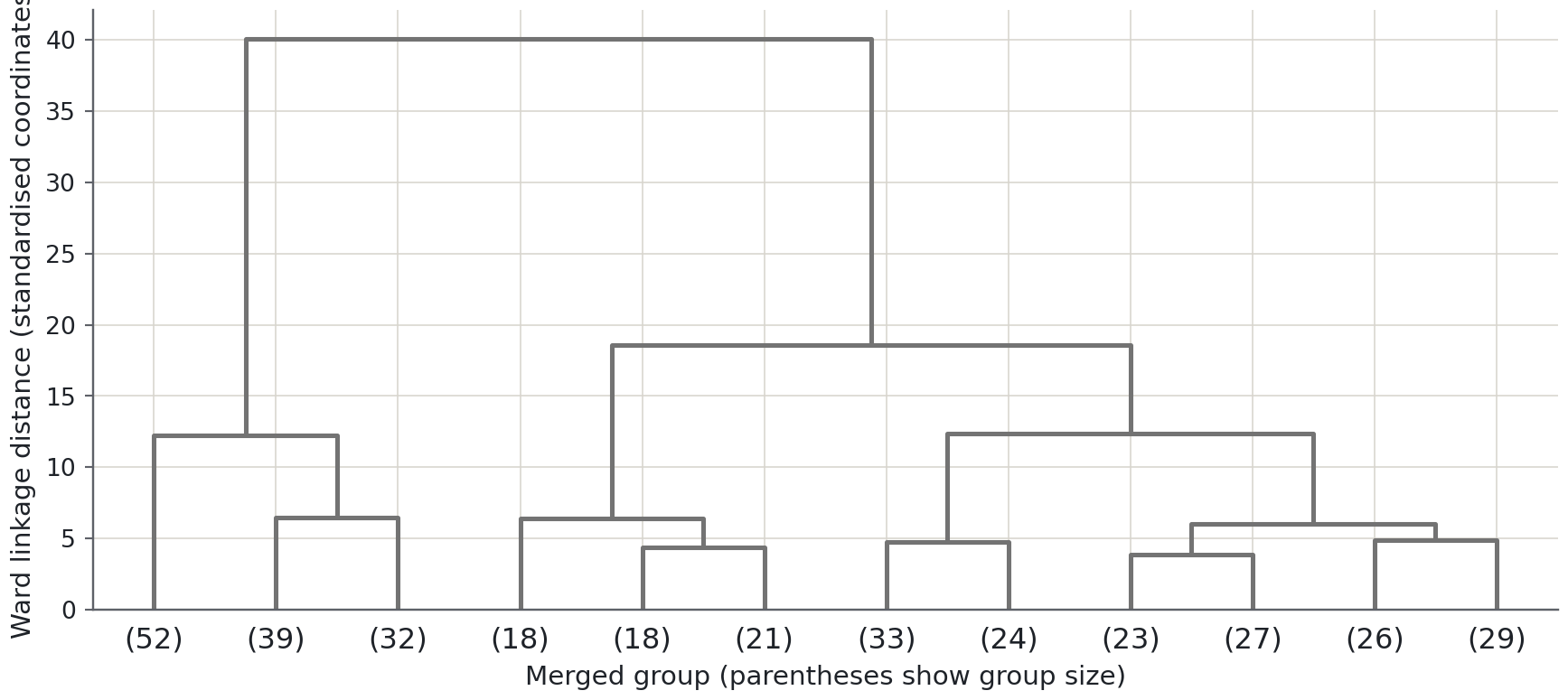
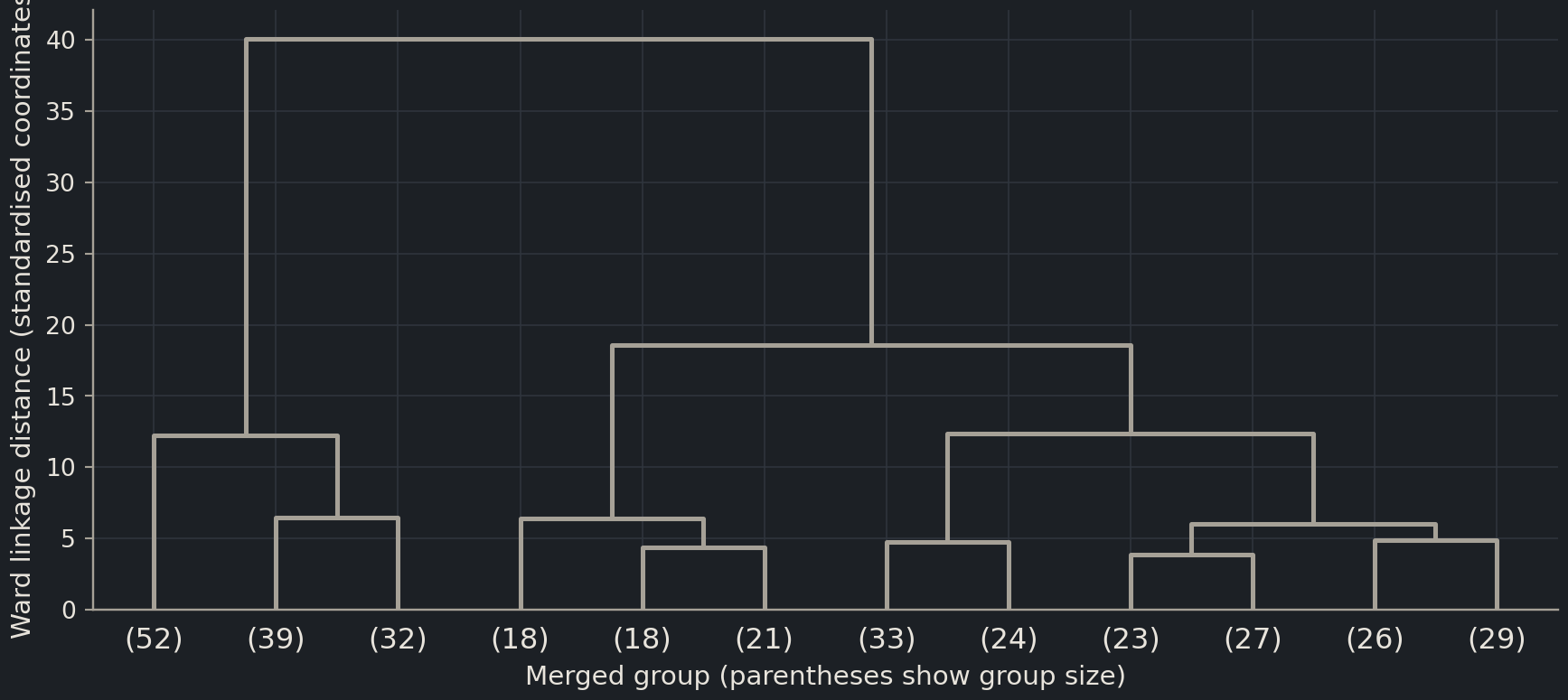
Agglomerative hierarchical clustering starts with separate observations and merges groups step by step. A dendrogramdendrogramA tree diagram showing the sequence and heights of hierarchical cluster merges. displays the sequence and the heights at which merges occur. The linkage rule determines what counts as a close pair of groups. Ward linkage, used here on Euclidean coordinates, favours merges that minimise the increase in within-cluster squared variation.
from scipy.cluster.hierarchy import dendrogram, linkagehierarchy = linkage(Z, method="ward")fig, ax = plt.subplots(figsize=(9, 4))dendrogram(hierarchy, truncate_mode="lastp", p=12, ax=ax, color_threshold=0, above_threshold_color="0.45")ax.set(xlabel="Merged group (parentheses show group size)", ylabel="Ward linkage distance (standardised coordinates)")plt.show()
Cutting this tree at different heights gives different partitions. A hierarchy is useful when groups plausibly contain subgroups, but it is still shaped by the chosen measurements and linkage. It is not an evolutionary phylogeny: its merge heights here reflect measurement distances, not time or ancestry.
Assigning a new observation is a separate promise
A fitted k-means object can assign a new observation to its nearest existing centre. To make that assignment comparable with the original table, transform the new measurements with the fitted scaler; do not estimate new means and scales from the incoming batch. The predicted cluster identifier refers to the original fitted partition, not to a new biological annotation supplied by the algorithm.
There is no automatic “none of the above” response in ordinary k-means. An animal far outside the observed range still receives the nearest cluster. If the application needs an unfamiliar-sample flag, inspect distances to centres and design a threshold on appropriate development data. Such a threshold answers a different question from choosing the number of clusters, and it needs evaluation on realistic unfamiliar examples.
Hierarchical clustering introduces another distinction: the fitted hierarchy describes relationships among the observations supplied during fitting. Adding observations and rebuilding the hierarchy can change existing merges. It does not automatically provide the same reusable predict rule as k-means. Decide whether your goal is to describe one collection or consistently assign future observations before choosing the workflow.
For stability, compare more than random initialisation. Refit on subsets of the development observations, then compare assignments for common rows or use a shared reference set where the method supports it. Ask whether broad groups persist when one correlated feature is omitted or reasonable scaling choices change. Report the perturbation and agreement measure instead of saying only that the clusters are “stable”. Stability to one perturbation establishes robustness to that perturbation; it cannot establish that the biological interpretation is correct.
Stability and alternatives
Repeat a declared clustering procedure after modest perturbations or on resampled observations. Compare whether the same samples stay together, accounting for arbitrary label numbering. Stable groups are more reproducible, but can still be stable artefacts. Inspect batch, collection site and missingness alongside the clusters.
K-means favours compact, roughly isotropic groups under Euclidean distance. Unequal densities, elongated shapes and outliers can make it a poor description. Density-based methods such as DBSCAN can identify non-spherical groups and noise, but introduce their own neighbourhood parameters and scale sensitivity. A Gaussian mixture allows overlapping probabilistic components with covariance structure, but its assumptions also need examination. Choose an algorithm from the scientific question and geometry, not from the most attractive plot.
Common mistake
Clusters are not automatically predictive classes
Calling cluster 2 “toxic” because several toxic examples appear there does not validate a toxicity classifier. Define the prediction task, reserve evaluation data and measure the proposed rule on independent labels. If cluster assignment becomes a predictive feature, fit the clustering transformation using only the training partition.
Exercises
Exercise★☆☆
A perfect inertia score
What happens if there is one centre for each distinct observation? Why is the resulting inertia unhelpful for choosing a scientific grouping?
SolutionShow solutionHide solution
Each observation can sit on a centre, giving zero inertia. This memorises the table and provides no useful compression or general grouping. Inertia must be interpreted together with complexity, stability and the purpose of the analysis.
Exercise★★☆
Compare partitions without comparing label numbers
Fit k-means with a second fixed seed and compare the assignments with the adjusted Rand index, which ignores arbitrary label numbering. What does a value of 1 establish, and what does it not establish?
SolutionShow solutionHide solution
from sklearn.metrics import adjusted_rand_scoreseed =7alternative = KMeans(n_clusters=3, n_init=10, random_state=seed).fit(Z)agreement = adjusted_rand_score(clusters.labels_, alternative.labels_)print(f"Adjusted Rand index between starts: {agreement:.3f}")
Adjusted Rand index between starts: 1.000
A value of 1 means the partitions match up to renaming clusters. It checks these two initialisation choices on the same table, not robustness to new samples, feature choices or biological validity. Do not keep trying seeds until one supports a preferred conclusion.
Where this is going
In Part III, clustering helps organise sequence and omics data, where batch effects and high-dimensional distances need particular care. Before moving there, model interpretation returns to supervised learning and asks what a successful prediction model actually relies on. Both activities turn an output into a scientific question rather than a final explanation.
Key points
A cluster depends on the representation, scaling, distance and algorithm.
K-means minimises within-cluster squared distance and prefers compact groups.
A high silhouette is evidence of separation under the chosen distance, not proof of a natural category.
Cluster identifiers are arbitrary; check stability, metadata and scientific meaning before naming groups.